Figure 1: A regular 3-layer Neural Network.

Artificial neural networks are computational systems that can learn to perform tasks by considering examples, generally without being programmed with any task-specific rules. It is supposed to mimic a biological system, wherein neurons interact by sending signals in the form of mathematical functions between layers. All layers can contain an arbitrary number of neurons, and each connection is represented by a weight variable.
The field of artificial neural networks has a long history of development, and is closely connected with the advancement of computer science and computers in general. A model of artificial neurons was first developed by McCulloch and Pitts in 1943 to study signal processing in the brain and has later been refined by others. The general idea is to mimic neural networks in the human brain, which is composed of billions of neurons that communicate with each other by sending electrical signals. Each neuron accumulates its incoming signals, which must exceed an activation threshold to yield an output. If the threshold is not overcome, the neuron remains inactive, i.e. has zero output.
This behaviour has inspired a simple mathematical model for an artificial neuron. $$ \begin{equation} y = f\left(\sum_{i=1}^n w_ix_i\right) = f(u) \label{artificialNeuron} \end{equation} $$ Here, the output \( y \) of the neuron is the value of its activation function, which have as input a weighted sum of signals \( x_i, \dots ,x_n \) received by \( n \) other neurons.
Conceptually, it is helpful to divide neural networks into four categories:
In quantum information theory, it has been shown that one can perform gate decompositions with the help of neural.
The applications are not limited to the natural sciences. There is a plethora of applications in essentially all disciplines, from the humanities to life science and medicine.
An artificial neural network (ANN), is a computational model that consists of layers of connected neurons, or nodes or units. We will refer to these interchangeably as units or nodes, and sometimes as neurons.
It is supposed to mimic a biological nervous system by letting each neuron interact with other neurons by sending signals in the form of mathematical functions between layers. A wide variety of different ANNs have been developed, but most of them consist of an input layer, an output layer and eventual layers in-between, called hidden layers. All layers can contain an arbitrary number of nodes, and each connection between two nodes is associated with a weight variable.
Neural networks (also called neural nets) are neural-inspired nonlinear models for supervised learning. As we will see, neural nets can be viewed as natural, more powerful extensions of supervised learning methods such as linear and logistic regression and soft-max methods we discussed earlier.
The feed-forward neural network (FFNN) was the first and simplest type of ANNs that were devised. In this network, the information moves in only one direction: forward through the layers.
Nodes are represented by circles, while the arrows display the connections between the nodes, including the direction of information flow. Additionally, each arrow corresponds to a weight variable (figure to come). We observe that each node in a layer is connected to all nodes in the subsequent layer, making this a so-called fully-connected FFNN.
A different variant of FFNNs are convolutional neural networks (CNNs), which have a connectivity pattern inspired by the animal visual cortex. Individual neurons in the visual cortex only respond to stimuli from small sub-regions of the visual field, called a receptive field. This makes the neurons well-suited to exploit the strong spatially local correlation present in natural images. The response of each neuron can be approximated mathematically as a convolution operation. (figure to come)
Convolutional neural networks emulate the behaviour of neurons in the visual cortex by enforcing a local connectivity pattern between nodes of adjacent layers: Each node in a convolutional layer is connected only to a subset of the nodes in the previous layer, in contrast to the fully-connected FFNN. Often, CNNs consist of several convolutional layers that learn local features of the input, with a fully-connected layer at the end, which gathers all the local data and produces the outputs. They have wide applications in image and video recognition.
So far we have only mentioned ANNs where information flows in one direction: forward. Recurrent neural networks on the other hand, have connections between nodes that form directed cycles. This creates a form of internal memory which are able to capture information on what has been calculated before; the output is dependent on the previous computations. Recurrent NNs make use of sequential information by performing the same task for every element in a sequence, where each element depends on previous elements. An example of such information is sentences, making recurrent NNs especially well-suited for handwriting and speech recognition.
There are many other kinds of ANNs that have been developed. One type that is specifically designed for interpolation in multidimensional space is the radial basis function (RBF) network. RBFs are typically made up of three layers: an input layer, a hidden layer with non-linear radial symmetric activation functions and a linear output layer (''linear'' here means that each node in the output layer has a linear activation function). The layers are normally fully-connected and there are no cycles, thus RBFs can be viewed as a type of fully-connected FFNN. They are however usually treated as a separate type of NN due the unusual activation functions.
One uses often so-called fully-connected feed-forward neural networks with three or more layers (an input layer, one or more hidden layers and an output layer) consisting of neurons that have non-linear activation functions.
Such networks are often called multilayer perceptrons (MLPs).
According to the Universal approximation theorem, a feed-forward neural network with just a single hidden layer containing a finite number of neurons can approximate a continuous multidimensional function to arbitrary accuracy, assuming the activation function for the hidden layer is a non-constant, bounded and monotonically-increasing continuous function.
Note that the requirements on the activation function only applies to the hidden layer, the output nodes are always assumed to be linear, so as to not restrict the range of output values.
The output \( y \) is produced via the activation function \( f \) $$ y = f\left(\sum_{i=1}^n w_ix_i + b_i\right) = f(z), $$ This function receives \( x_i \) as inputs. Here the activation \( z=(\sum_{i=1}^n w_ix_i+b_i) \). In an FFNN of such neurons, the inputs \( x_i \) are the outputs of the neurons in the preceding layer. Furthermore, an MLP is fully-connected, which means that each neuron receives a weighted sum of the outputs of all neurons in the previous layer.
First, for each node \( i \) in the first hidden layer, we calculate a weighted sum \( z_i^1 \) of the input coordinates \( x_j \), $$ \begin{equation} z_i^1 = \sum_{j=1}^{M} w_{ij}^1 x_j + b_i^1 \label{_auto1} \end{equation} $$
Here \( b_i \) is the so-called bias which is normally needed in case of zero activation weights or inputs. How to fix the biases and the weights will be discussed below. The value of \( z_i^1 \) is the argument to the activation function \( f_i \) of each node \( i \), The variable \( M \) stands for all possible inputs to a given node \( i \) in the first layer. We define the output \( y_i^1 \) of all neurons in layer 1 as $$ \begin{equation} y_i^1 = f(z_i^1) = f\left(\sum_{j=1}^M w_{ij}^1 x_j + b_i^1\right) \label{outputLayer1} \end{equation} $$
where we assume that all nodes in the same layer have identical activation functions, hence the notation \( f \). In general, we could assume in the more general case that different layers have different activation functions. In this case we would identify these functions with a superscript \( l \) for the \( l \)-th layer, $$ \begin{equation} y_i^l = f^l(u_i^l) = f^l\left(\sum_{j=1}^{N_{l-1}} w_{ij}^l y_j^{l-1} + b_i^l\right) \label{generalLayer} \end{equation} $$
where \( N_l \) is the number of nodes in layer \( l \). When the output of all the nodes in the first hidden layer are computed, the values of the subsequent layer can be calculated and so forth until the output is obtained.
The output of neuron \( i \) in layer 2 is thus, $$ \begin{align} y_i^2 &= f^2\left(\sum_{j=1}^N w_{ij}^2 y_j^1 + b_i^2\right) \label{_auto2}\\ &= f^2\left[\sum_{j=1}^N w_{ij}^2f^1\left(\sum_{k=1}^M w_{jk}^1 x_k + b_j^1\right) + b_i^2\right] \label{outputLayer2} \end{align} $$ where we have substituted \( y_k^1 \) with the inputs \( x_k \). Finally, the ANN output reads $$ \begin{align} y_i^3 &= f^3\left(\sum_{j=1}^N w_{ij}^3 y_j^2 + b_i^3\right) \label{_auto3}\\ &= f_3\left[\sum_{j} w_{ij}^3 f^2\left(\sum_{k} w_{jk}^2 f^1\left(\sum_{m} w_{km}^1 x_m + b_k^1\right) + b_j^2\right) + b_1^3\right] \label{_auto4} \end{align} $$
We can generalize this expression to an MLP with \( l \) hidden layers. The complete functional form is, $$ \begin{align} &y^{l+1}_i = f^{l+1}\left[\!\sum_{j=1}^{N_l} w_{ij}^3 f^l\left(\sum_{k=1}^{N_{l-1}}w_{jk}^{l-1}\left(\dots f^1\left(\sum_{n=1}^{N_0} w_{mn}^1 x_n+ b_m^1\right)\dots\right)+b_k^2\right)+b_1^3\right] && \label{completeNN} \end{align} $$
which illustrates a basic property of MLPs: The only independent variables are the input values \( x_n \).
This confirms that an MLP, despite its quite convoluted mathematical form, is nothing more than an analytic function, specifically a mapping of real-valued vectors \( \hat{x} \in \mathbb{R}^n \rightarrow \hat{y} \in \mathbb{R}^m \).
Furthermore, the flexibility and universality of an MLP can be illustrated by realizing that the expression is essentially a nested sum of scaled activation functions of the form $$ \begin{equation} f(x) = c_1 f(c_2 x + c_3) + c_4 \label{_auto5} \end{equation} $$
where the parameters \( c_i \) are weights and biases. By adjusting these parameters, the activation functions can be shifted up and down or left and right, change slope or be rescaled which is the key to the flexibility of a neural network.
We can introduce a more convenient notation for the activations in an A NN.
Additionally, we can represent the biases and activations as layer-wise column vectors \( \hat{b}_l \) and \( \hat{y}_l \), so that the \( i \)-th element of each vector is the bias \( b_i^l \) and activation \( y_i^l \) of node \( i \) in layer \( l \) respectively.
We have that \( \mathrm{W}_l \) is an \( N_{l-1} \times N_l \) matrix, while \( \hat{b}_l \) and \( \hat{y}_l \) are \( N_l \times 1 \) column vectors. With this notation, the sum becomes a matrix-vector multiplication, and we can write the equation for the activations of hidden layer 2 (assuming three nodes for simplicity) as $$ \begin{equation} \hat{y}_2 = f_2(\mathrm{W}_2 \hat{y}_{1} + \hat{b}_{2}) = f_2\left(\left[\begin{array}{ccc} w^2_{11} &w^2_{12} &w^2_{13} \\ w^2_{21} &w^2_{22} &w^2_{23} \\ w^2_{31} &w^2_{32} &w^2_{33} \\ \end{array} \right] \cdot \left[\begin{array}{c} y^1_1 \\ y^1_2 \\ y^1_3 \\ \end{array}\right] + \left[\begin{array}{c} b^2_1 \\ b^2_2 \\ b^2_3 \\ \end{array}\right]\right). \label{_auto6} \end{equation} $$
The activation of node \( i \) in layer 2 is $$ \begin{equation} y^2_i = f_2\Bigr(w^2_{i1}y^1_1 + w^2_{i2}y^1_2 + w^2_{i3}y^1_3 + b^2_i\Bigr) = f_2\left(\sum_{j=1}^3 w^2_{ij} y_j^1 + b^2_i\right). \label{_auto7} \end{equation} $$
This is not just a convenient and compact notation, but also a useful and intuitive way to think about MLPs: The output is calculated by a series of matrix-vector multiplications and vector additions that are used as input to the activation functions. For each operation \( \mathrm{W}_l \hat{y}_{l-1} \) we move forward one layer.
A property that characterizes a neural network, other than its connectivity, is the choice of activation function(s). As described in, the following restrictions are imposed on an activation function for a FFNN to fulfill the universal approximation theorem
The second requirement excludes all linear functions. Furthermore, in a MLP with only linear activation functions, each layer simply performs a linear transformation of its inputs.
Regardless of the number of layers, the output of the NN will be nothing but a linear function of the inputs. Thus we need to introduce some kind of non-linearity to the NN to be able to fit non-linear functions Typical examples are the logistic Sigmoid $$ f(x) = \frac{1}{1 + e^{-x}}, $$ and the hyperbolic tangent function $$ f(x) = \tanh(x) $$
The sigmoid function are more biologically plausible because the output of inactive neurons are zero. Such activation function are called one-sided. However, it has been shown that the hyperbolic tangent performs better than the sigmoid for training MLPs. has become the most popular for deep neural networks
"""The sigmoid function (or the logistic curve) is a
function that takes any real number, z, and outputs a number (0,1).
It is useful in neural networks for assigning weights on a relative scale.
The value z is the weighted sum of parameters involved in the learning algorithm."""

import numpy
import matplotlib.pyplot as plt
import math as mt

z = numpy.arange(-5, 5, .1)
sigma_fn = numpy.vectorize(lambda z: 1/(1+numpy.exp(-z)))
sigma = sigma_fn(z)

fig = plt.figure()
ax = fig.add_subplot(111)
ax.plot(z, sigma)
ax.set_ylim([-0.1, 1.1])
ax.set_xlim([-5,5])
ax.grid(True)
ax.set_xlabel('z')
ax.set_title('sigmoid function')

plt.show()

"""Step Function"""
z = numpy.arange(-5, 5, .02)
step_fn = numpy.vectorize(lambda z: 1.0 if z >= 0.0 else 0.0)
step = step_fn(z)

fig = plt.figure()
ax = fig.add_subplot(111)
ax.plot(z, step)
ax.set_ylim([-0.5, 1.5])
ax.set_xlim([-5,5])
ax.grid(True)
ax.set_xlabel('z')
ax.set_title('step function')

plt.show()

"""Sine Function"""
z = numpy.arange(-2*mt.pi, 2*mt.pi, 0.1)
t = numpy.sin(z)

fig = plt.figure()
ax = fig.add_subplot(111)
ax.plot(z, t)
ax.set_ylim([-1.0, 1.0])
ax.set_xlim([-2*mt.pi,2*mt.pi])
ax.grid(True)
ax.set_xlabel('z')
ax.set_title('sine function')

plt.show()

"""Plots a graph of the squashing function used by a rectified linear
unit"""
z = numpy.arange(-2, 2, .1)
zero = numpy.zeros(len(z))
y = numpy.max([zero, z], axis=0)

fig = plt.figure()
ax = fig.add_subplot(111)
ax.plot(z, y)
ax.set_ylim([-2.0, 2.0])
ax.set_xlim([-2.0, 2.0])
ax.grid(True)
ax.set_xlabel('z')
ax.set_title('Rectified linear unit')

plt.show()
The multilayer perceptron is a very popular, and easy to implement approach, to deep learning. It consists of
For an MLP network there is no direct connection between the output nodes/neurons/units and the input nodes/neurons/units. Hereafter we will call the various entities of a layer for nodes. There are also no connections within a single layer.
The number of input nodes does not need to equal the number of output nodes. This applies also to the hidden layers. Each layer may have its own number of nodes and activation functions.
The hidden layers have their name from the fact that they are not linked to observables and as we will see below when we define the so-called activation \( \hat{z} \), we can think of this as a basis expansion of the original inputs \( \hat{x} \). The difference however between neural networks and say linear regression is that now these basis functions (which will correspond to the weights in the network) are learned from data. This results in an important difference between neural networks and deep learning approaches on one side and methods like logistic regression or linear regression and their modifications on the other side.
A neural network with only one layer, what we called the simple perceptron, is best suited if we have a standard binary model with clear (linear) boundaries between the outcomes. As such it could equally well be replaced by standard linear regression or logistic regression. Networks with one or more hidden layers approximate systems with more complex boundaries.
As stated earlier, an important theorem in studies of neural networks, restated without proof here, is the universal approximation theorem.
It states that a feed-forward network with a single hidden layer containing a finite number of neurons can approximate continuous functions on compact subsets of real functions. The theorem thus states that simple neural networks can represent a wide variety of interesting functions when given appropriate parameters. It is the multilayer feedforward architecture itself which gives neural networks the potential of being universal approximators.
Note: figures will be inserted later!
As we have seen now in a feed forward network, we can express the final output of our network in terms of basic matrix-vector multiplications. The unknowwn quantities are our weights \( w_{ij} \) and we need to find an algorithm for changing them so that our errors are as small as possible. This leads us to the famous back propagation algorithm.
The questions we want to ask are how do changes in the biases and the weights in our network change the cost function and how can we use the final output to modify the weights?
To derive these equations let us start with a plain regression problem and define our cost function as $$ {\cal C}(\hat{W}) = \frac{1}{2}\sum_{i=1}^n\left(y_i - t_i\right)^2, $$
where the $t_i$s are our \( n \) targets (the values we want to reproduce), while the outputs of the network after having propagated all inputs \( \hat{x} \) are given by \( y_i \). Below we will demonstrate how the basic equations arising from the back propagation algorithm can be modified in order to study classification problems with \( K \) classes.
With our definition of the targets \( \hat{t} \), the outputs of the network \( \hat{y} \) and the inputs \( \hat{x} \) we define now the activation \( z_j^l \) of node/neuron/unit \( j \) of the \( l \)-th layer as a function of the bias, the weights which add up from the previous layer \( l-1 \) and the forward passes/outputs \( \hat{a}^{l-1} \) from the previous layer as $$ z_j^l = \sum_{i=1}^{M_{l-1}}w_{ij}^la_i^{l-1}+b_j^l, $$
where \( b_k^l \) are the biases from layer \( l \). Here \( M_{l-1} \) represents the total number of nodes/neurons/units of layer \( l-1 \). The figure here illustrates this equation. We can rewrite this in a more compact form as the matrix-vector products we discussed earlier, $$ \hat{z}^l = \left(\hat{W}^l\right)^T\hat{a}^{l-1}+\hat{b}^l. $$
With the activation values \( \hat{z}^l \) we can in turn define the output of layer \( l \) as \( \hat{a}^l = f(\hat{z}^l) \) where \( f \) is our activation function. In the examples here we will use the sigmoid function discussed in our logistic regression lectures. We will also use the same activation function \( f \) for all layers and their nodes. It means we have $$ a_j^l = f(z_j^l) = \frac{1}{1+\exp{-(z_j^l)}}. $$
From the definition of the activation \( z_j^l \) we have $$ \frac{\partial z_j^l}{\partial w_{ij}^l} = a_i^{l-1}, $$ and $$ \frac{\partial z_j^l}{\partial a_i^{l-1}} = w_{ji}^l. $$
With our definition of the activation function we have that (note that this function depends only on \( z_j^l \)) $$ \frac{\partial a_j^l}{\partial z_j^{l}} = a_j^l(1-a_j^l)=f(z_j^l)(1-f(z_j^l)). $$
With these definitions we can now compute the derivative of the cost function in terms of the weights.
Let us specialize to the output layer \( l=L \). Our cost function is $$ {\cal C}(\hat{W^L}) = \frac{1}{2}\sum_{i=1}^n\left(y_i - t_i\right)^2=\frac{1}{2}\sum_{i=1}^n\left(a_i^L - t_i\right)^2, $$ The derivative of this function with respect to the weights is $$ \frac{\partial{\cal C}(\hat{W^L})}{\partial w_{jk}^L} = \left(a_j^L - t_j\right)\frac{\partial a_j^L}{\partial w_{jk}^{L}}, $$ The last partial derivative can easily be computed and reads (by applying the chain rule) $$ \frac{\partial a_j^L}{\partial w_{jk}^{L}} = \frac{\partial a_j^L}{\partial z_{j}^{L}}\frac{\partial z_j^L}{\partial w_{jk}^{L}}=a_j^L(1-a_j^L)a_k^{L-1}, $$
We have thus $$ \frac{\partial{\cal C}(\hat{W^L})}{\partial w_{jk}^L} = \left(a_j^L - t_j\right)a_j^L(1-a_j^L)a_k^{L-1}, $$
Defining $$ \delta_j^L = a_j^L(1-a_j^L)\left(a_j^L - t_j\right) = f'(z_j^L)\frac{\partial {\cal C}}{\partial (a_j^L)}, $$ and using the Hadamard product of two vectors we can write this as $$ \hat{\delta}^L = f'(\hat{z}^L)\circ\frac{\partial {\cal C}}{\partial (\hat{a}L)}. $$
This is an important expression. The second term on the right handside measures how fast the cost function is changing as a function of the $j$th output activation. If, for example, the cost function doesn't depend much on a particular output node \( j \), then \( \delta_j^L \) will be small, which is what we would expect. The first term on the right, measures how fast the activation function \( f \) is changing at a given activation value \( z_j^L \).
Notice that everything in the above equations is easily computed. In particular, we compute \( z_j^L \) while computing the behaviour of the network, and it is only a small additional overhead to compute \( f'(z^L_j) \). The exact form of the derivative with respect to the output depends on the form of the cost function. However, provided the cost function is known there should be little trouble in calculating $$ \frac{\partial {\cal C}}{\partial (a_j^L)} $$
With the definition of \( \delta_j^L \) we have a more compact definition of the derivative of the cost function in terms of the weights, namely $$ \frac{\partial{\cal C}(\hat{W^L})}{\partial w_{jk}^L} = \delta_j^La_k^{L-1}. $$
It is also easy to see that our previous equation can be written as
$$
\delta_j^L =\frac{\partial {\cal C}}{\partial z_j^L}= \frac{\partial {\cal C}}{\partial a_j^L}\frac{\partial a_j^L}{\partial z_j^L},
$$
which can also be interpreted as the partial derivative of the cost function with respect to the biases \( b_j^L \), namely
$$
\delta_j^L = \frac{\partial {\cal C}}{\partial b_j^L}\frac{\partial b_j^L}{\partial z_j^L}=\frac{\partial {\cal C}}{\partial b_j^L},
$$
That is, the error \( \delta_j^L \) is exactly equal to the rate of change of the cost function as a function of the bias.
We have now three equations that are essential for the computations of the derivatives of the cost function at the output layer. These equations are needed to start the algorithm and they are
$$ \begin{equation} \frac{\partial{\cal C}(\hat{W^L})}{\partial w_{jk}^L} = \delta_j^La_k^{L-1}, \label{_auto8} \end{equation} $$ and $$ \begin{equation} \delta_j^L = f'(z_j^L)\frac{\partial {\cal C}}{\partial (a_j^L)}, \label{_auto9} \end{equation} $$ and $$ \begin{equation} \delta_j^L = \frac{\partial {\cal C}}{\partial b_j^L}, \label{_auto10} \end{equation} $$
An interesting consequence of the above equations is that when the activation \( a_k^{L-1} \) is small, the gradient term, that is the derivative of the cost function with respect to the weights, will also tend to be small. We say then that the weight learns slowly, meaning that it changes slowly when we minimize the weights via say gradient descent. In this case we say the system learns slowly.
Another interesting feature is that is when the activation function, represented by the sigmoid function here, is rather flat when we move towards its end values \( 0 \) and \( 1 \) (see the above Python codes). In these cases, the derivatives of the activation function will also be close to zero, meaning again that the gradients will be small and the network learns slowly again.
We need a fourth equation and we are set. We are going to propagate backwards in order to the determine the weights and biases. In order to do so we need to represent the error in the layer before the final one \( L-1 \) in terms of the errors in the final output layer.
We have that (replacing \( L \) with a general layer \( l \)) $$ \delta_j^l =\frac{\partial {\cal C}}{\partial z_j^l}. $$ We want to express this in terms of the equations for layer \( l+1 \). Using the chain rule and summing over all \( k \) entries we have $$ \delta_j^l =\sum_k \frac{\partial {\cal C}}{\partial z_k^{l+1}}\frac{\partial z_k^{l+1}}{\partial z_j^{l}}=\sum_k \delta_k^{l+1}\frac{\partial z_k^{l+1}}{\partial z_j^{l}}, $$ and recalling that $$ z_j^{l+1} = \sum_{i=1}^{M_{l}}w_{ij}^{l+1}a_j^{l}+b_j^{l+1}, $$ with \( M_l \) being the number of nodes in layer \( l \), we obtain $$ \delta_j^l =\sum_k \delta_k^{l+1}w_{kj}^{l+1}f'(z_j^l), $$ This is our final equation.
We are now ready to set up the algorithm for back propagation and learning the weights and biases.
The four equations provide us with a way of computing the gradient of the cost function. Let us write this out in the form of an algorithm.
First, we set up the input data \( \hat{x} \) and the activations \( \hat{z}_1 \) of the input layer and compute the activation function and the pertinent outputs \( \hat{a}^1 \).
Secondly, we perform then the feed forward till we reach the output layer and compute all \( \hat{z}_l \) of the input layer and compute the activation function and the pertinent outputs \( \hat{a}^l \) for \( l=2,3,\dots,L \).
Thereafter we compute the ouput error \( \hat{\delta}^L \) by computing all $$ \delta_j^L = f'(z_j^L)\frac{\partial {\cal C}}{\partial (a_j^L)}. $$
Then we compute the back propagate error for each \( l=L-1,L-2,\dots,2 \) as $$ \delta_j^l = \sum_k \delta_k^{l+1}w_{kj}^{l+1}f'(z_j^l). $$
Finally, we update the weights and the biases using gradient descent for each \( l=L-1,L-2,\dots,2 \) and update the weights and biases according to the rules $$ w_{jk}^l\leftarrow = w_{jk}^l- \eta \delta_j^la_k^{l-1}, $$ $$ b_j^l \leftarrow b_j^l-\eta \frac{\partial {\cal C}}{\partial b_j^l}=b_j^l-\eta \delta_j^l, $$
The parameter \( \eta \) is the learning parameter discussed in connection with the gradient descent methods. Here it is convenient to use stochastic gradient descent (see the examples below) with mini-batches with an outer loop that steps through multiple epochs of training.
We are now gong to develop an example based on the MNIST data base. This is a classification problem and we need to use our cross-entropy function we discussed in connection with logistic regression. The cross-entropy defines our cost function for the classificaton problems with neural networks.
In binary classification with two classes \( (0, 1) \) we define the logistic/sigmoid function as the probability that a particular input is in class \( 0 \) or \( 1 \). This is possible because the logistic function takes any input from the real numbers and inputs a number between 0 and 1, and can therefore be interpreted as a probability. It also has other nice properties, such as a derivative that is simple to calculate.
For an input \( \boldsymbol{a} \) from the hidden layer, the probability that the input \( \boldsymbol{x} \) is in class 0 or 1 is just. We let \( \theta \) represent the unknown weights and biases to be adjusted by our equations). The variable \( x \) represents our activation values \( z \). We have $$ P(y = 0 \mid \hat{x}, \hat{\theta}) = \frac{1}{1 + \exp{(- \hat{x}})} , $$ and $$ P(y = 1 \mid \hat{x}, \hat{\theta}) = 1 - P(y = 0 \mid \hat{x}, \hat{\theta}) , $$
where \( y \in \{0, 1\} \) and \( \hat{\theta} \) represents the weights and biases of our network.
Our cost function is given as (see the Logistic regression lectures) $$ \mathcal{C}(\hat{\theta}) = - \ln P(\mathcal{D} \mid \hat{\theta}) = - \sum_{i=1}^n y_i \ln[P(y_i = 0)] + (1 - y_i) \ln [1 - P(y_i = 0)] = \sum_{i=1}^n \mathcal{L}_i(\hat{\theta}) . $$
This last equality means that we can interpret our cost function as a sum over the loss function for each point in the dataset \( \mathcal{L}_i(\hat{\theta}) \). The negative sign is just so that we can think about our algorithm as minimizing a positive number, rather than maximizing a negative number.
In multiclass classification it is common to treat each integer label as a so called one-hot vector:
\( y = 5 \quad \rightarrow \quad \hat{y} = (0, 0, 0, 0, 0, 1, 0, 0, 0, 0) , \) and
\( y = 1 \quad \rightarrow \quad \hat{y} = (0, 1, 0, 0, 0, 0, 0, 0, 0, 0) , \)
i.e. a binary bit string of length \( C \), where \( C = 10 \) is the number of classes in the MNIST dataset (numbers from \( 0 \) to \( 9 \))..
If \( \hat{x}_i \) is the \( i \)-th input (image), \( y_{ic} \) refers to the \( c \)-th component of the \( i \)-th output vector \( \hat{y}_i \). The probability of \( \hat{x}_i \) being in class \( c \) will be given by the softmax function: $$ P(y_{ic} = 1 \mid \hat{x}_i, \hat{\theta}) = \frac{\exp{((\hat{a}_i^{hidden})^T \hat{w}_c)}} {\sum_{c'=0}^{C-1} \exp{((\hat{a}_i^{hidden})^T \hat{w}_{c'})}} , $$
which reduces to the logistic function in the binary case. The likelihood of this \( C \)-class classifier is now given as: $$ P(\mathcal{D} \mid \hat{\theta}) = \prod_{i=1}^n \prod_{c=0}^{C-1} [P(y_{ic} = 1)]^{y_{ic}} . $$ Again we take the negative log-likelihood to define our cost function: $$ \mathcal{C}(\hat{\theta}) = - \log{P(\mathcal{D} \mid \hat{\theta})}. $$ See the logistic regression lectures for a full definition of the cost function.
The back propagation equations need now only a small change, namely the definition of a new cost function. We are thus ready to use the same equations as before!
As an example of the above, relevant for project 2 as well, let us consider a binary class. As discussed in our logistic regression lectures, we defined a cost function in terms of the parameters \( \beta \) as $$ \mathcal{C}(\hat{\beta}) = - \sum_{i=1}^n \left(y_i\log{p(y_i \vert x_i,\hat{\beta})}+(i-y_i)\log{1-p(y_i \vert x_i,\hat{\beta})}\right), $$ where we had defined the logistic (sigmoid) function $$ p(y_i =1\vert x_i,\hat{\beta})=\frac{\exp{(\beta_0+\beta_1 x_i)}}{1+\exp{(\beta_0+\beta_1 x_i)}}, $$ and $$ p(y_i =0\vert x_i,\hat{\beta})=1-p(y_i =1\vert x_i,\hat{\beta}). $$ The parameters \( \hat{\beta} \) were defined using a minimization method like gradient descent or Newton-Raphson's method.
Now we replace \( x_i \) with the activation \( z_i^l \) for a given layer \( l \) and the outputs as \( y_i=a_i^l=f(z_i^l) \), with \( z_i^l \) now being a function of the weights \( w_{ij}^l \) and biases \( b_i^l \). We have then $$ a_i^l = y_i = \frac{\exp{(z_i^l)}}{1+\exp{(z_i^l)}}, $$ with $$ z_i^l = \sum_{j}w_{ij}^l a_j^{l-1}+b_i^l, $$ where the superscript \( l-1 \) indicates that these are the outputs from layer \( l-1 \). Our cost function at the final layer \( l=L \) is now $$ \mathcal{C}(\hat{W}) = - \sum_{i=1}^n \left(t_i\log{a_i^L}+(1-t_i)\log{(1-a_i^L)}\right), $$ where we have defined the targets \( t_i \). The derivatives of the cost function with respect to the output \( a_i^L \) are then easily calculated and we get $$ \frac{\partial \mathcal{C}(\hat{W})}{\partial a_i^L} = \frac{a_i^L-t_i}{a_i^L(1-a_i^L)}. $$ In case we use another activation function than the logistic one, we need to evaluate other derivatives.
One can identify a set of key steps when using neural networks to solve supervised learning problems:
Here we will be using the MNIST dataset, which is readily available through the scikit-learn package. You may also find it for example here. The MNIST (Modified National Institute of Standards and Technology) database is a large database of handwritten digits that is commonly used for training various image processing systems. The MNIST dataset consists of 70 000 images of size \( 28\times 28 \) pixels, each labeled from 0 to 9. The scikit-learn dataset we will use consists of a selection of 1797 images of size \( 8\times 8 \) collected and processed from this database.
To feed data into a feed-forward neural network we need to represent the inputs as a feature matrix \( X = (n_{inputs}, n_{features}) \). Each row represents an input, in this case a handwritten digit, and each column represents a feature, in this case a pixel. The correct answers, also known as labels or targets are represented as a 1D array of integers \( Y = (n_{inputs}) = (5, 3, 1, 8,...) \).
As an example, say we want to build a neural network using supervised learning to predict Body-Mass Index (BMI) from measurements of height (in m) and weight (in kg). If we have measurements of 5 people the feature matrix could be for example: $$ X = \begin{bmatrix} 1.85 & 81\\ 1.71 & 65\\ 1.95 & 103\\ 1.55 & 42\\ 1.63 & 56 \end{bmatrix} ,$$
and the targets would be: $$ Y = (23.7, 22.2, 27.1, 17.5, 21.1) $$
Since each input image is a 2D matrix, we need to flatten the image (i.e. "unravel" the 2D matrix into a 1D array) to turn the data into a feature matrix. This means we lose all spatial information in the image, such as locality and translational invariance. More complicated architectures such as Convolutional Neural Networks can take advantage of such information, and are most commonly applied when analyzing images.
# import necessary packages
import numpy as np
import matplotlib.pyplot as plt
from sklearn import datasets


# ensure the same random numbers appear every time
np.random.seed(0)

# display images in notebook
%matplotlib inline
plt.rcParams['figure.figsize'] = (12,12)


# download MNIST dataset
digits = datasets.load_digits()

# define inputs and labels
inputs = digits.images
labels = digits.target

print("inputs = (n_inputs, pixel_width, pixel_height) = " + str(inputs.shape))
print("labels = (n_inputs) = " + str(labels.shape))


# flatten the image
# the value -1 means dimension is inferred from the remaining dimensions: 8x8 = 64
n_inputs = len(inputs)
inputs = inputs.reshape(n_inputs, -1)
print("X = (n_inputs, n_features) = " + str(inputs.shape))


# choose some random images to display
indices = np.arange(n_inputs)
random_indices = np.random.choice(indices, size=5)

for i, image in enumerate(digits.images[random_indices]):
    plt.subplot(1, 5, i+1)
    plt.axis('off')
    plt.imshow(image, cmap=plt.cm.gray_r, interpolation='nearest')
    plt.title("Label: %d" % digits.target[random_indices[i]])
plt.show()
Performing analysis before partitioning the dataset is a major error, that can lead to incorrect conclusions.
We will reserve \( 80 \% \) of our dataset for training and \( 20 \% \) for testing.
It is important that the train and test datasets are drawn randomly from our dataset, to ensure no bias in the sampling. Say you are taking measurements of weather data to predict the weather in the coming 5 days. You don't want to train your model on measurements taken from the hours 00.00 to 12.00, and then test it on data collected from 12.00 to 24.00.
from sklearn.model_selection import train_test_split

# one-liner from scikit-learn library
train_size = 0.8
test_size = 1 - train_size
X_train, X_test, Y_train, Y_test = train_test_split(inputs, labels, train_size=train_size,
                                                    test_size=test_size)

# equivalently in numpy
def train_test_split_numpy(inputs, labels, train_size, test_size):
    n_inputs = len(inputs)
    inputs_shuffled = inputs.copy()
    labels_shuffled = labels.copy()

    np.random.shuffle(inputs_shuffled)
    np.random.shuffle(labels_shuffled)

    train_end = int(n_inputs*train_size)
    X_train, X_test = inputs_shuffled[:train_end], inputs_shuffled[train_end:]
    Y_train, Y_test = labels_shuffled[:train_end], labels_shuffled[train_end:]

    return X_train, X_test, Y_train, Y_test

#X_train, X_test, Y_train, Y_test = train_test_split_numpy(inputs, labels, train_size, test_size)

print("Number of training images: " + str(len(X_train)))
print("Number of test images: " + str(len(X_test)))
Our simple feed-forward neural network will consist of an input layer, a single hidden layer and an output layer. The activation \( y \) of each neuron is a weighted sum of inputs, passed through an activation function. In case of the simple perceptron model we have $$ z = \sum_{i=1}^n w_i a_i ,$$ $$ y = f(z) ,$$
where \( f \) is the activation function, \( a_i \) represents input from neuron \( i \) in the preceding layer and \( w_i \) is the weight to input \( i \). The activation of the neurons in the input layer is just the features (e.g. a pixel value).
The simplest activation function for a neuron is the Heaviside function: $$ f(z) = \begin{cases} 1, & z > 0\\ 0, & \text{otherwise} \end{cases} $$
A feed-forward neural network with this activation is known as a perceptron. For a binary classifier (i.e. two classes, 0 or 1, dog or not-dog) we can also use this in our output layer. This activation can be generalized to \( k \) classes (using e.g. the one-against-all strategy), and we call these architectures multiclass perceptrons.
However, it is now common to use the terms Single Layer Perceptron (SLP) (1 hidden layer) and Multilayer Perceptron (MLP) (2 or more hidden layers) to refer to feed-forward neural networks with any activation function.
Typical choices for activation functions include the sigmoid function, hyperbolic tangent, and Rectified Linear Unit (ReLU). We will be using the sigmoid function \( \sigma(x) \): $$ f(x) = \sigma(x) = \frac{1}{1 + e^{-x}} ,$$
which is inspired by probability theory (see logistic regression) and was most commonly used until about 2011. See the discussion below concerning other activation functions.
For a soft binary classifier, we could use a single neuron and interpret the output as either being the probability of being in class 0 or the probability of being in class 1. Alternatively we could use 2 neurons, and interpret each neuron as the probability of being in each class.
Since we are doing multiclass classification, with 10 categories, it is natural to use 10 neurons in the output layer. We number the neurons \( j = 0,1,...,9 \). The activation of each output neuron \( j \) will be according to the softmax function: $$ P(\text{class \( j \)} \mid \text{input \( \hat{a} \)}) = \frac{\exp{(\hat{a}^T \hat{w}_j)}} {\sum_{c=0}^{9} \exp{(\hat{a}^T \hat{w}_c)}} ,$$
i.e. each neuron \( j \) outputs the probability of being in class \( j \) given an input from the hidden layer \( \hat{a} \), with \( \hat{w}_j \) the weights of neuron \( j \) to the inputs. The denominator is a normalization factor to ensure the outputs (probabilities) sum up to 1. The exponent is just the weighted sum of inputs as before: $$ z_j = \sum_{i=1}^n w_ {ij} a_i+b_j.$$
Since each neuron in the output layer is connected to the 50 inputs from the hidden layer we have 50x10 = 500 weights to the output layer.
Typically weights are initialized with small values distributed around zero, drawn from a uniform or normal distribution. Setting all weights to zero means all neurons give the same output, making the network useless.
Adding a bias value to the weighted sum of inputs allows the neural network to represent a greater range of values. Without it, any input with the value 0 will be mapped to zero (before being passed through the activation). The bias unit has an output of 1, and a weight to each neuron \( j \), \( b_j \): $$ z_j = \sum_{i=1}^n w_ {ij} a_i + b_j.$$
The bias weights \( \hat{b} \) are often initialized to zero, but a small value like \( 0.01 \) ensures all neurons have some output which can be backpropagated in the first training cycle.
# building our neural network

n_inputs, n_features = X_train.shape
n_hidden_neurons = 50
n_categories = 10

# we make the weights normally distributed using numpy.random.randn

# weights and bias in the hidden layer
hidden_weights = np.random.randn(n_features, n_hidden_neurons)
hidden_bias = np.zeros(n_hidden_neurons) + 0.01

# weights and bias in the output layer
output_weights = np.random.randn(n_hidden_neurons, n_categories)
output_bias = np.zeros(n_categories) + 0.01
Denote \( F \) the number of features, \( H \) the number of hidden neurons and \( C \) the number of categories. For each input image we calculate a weighted sum of input features (pixel values) to each neuron \( j \) in the hidden layer \( l \): $$ z_{j}^{l} = \sum_{i=1}^{F} w_{ij}^{l} x_i + b_{j}^{l},$$
this is then passed through our activation function $$ a_{j}^{l} = f(z_{j}^{l}) .$$
We calculate a weighted sum of inputs (activations in the hidden layer) to each neuron \( j \) in the output layer: $$ z_{j}^{L} = \sum_{i=1}^{H} w_{ij}^{L} a_{i}^{l} + b_{j}^{L}.$$
Finally we calculate the output of neuron \( j \) in the output layer using the softmax function: $$ a_{j}^{L} = \frac{\exp{(z_j^{L})}} {\sum_{c=0}^{C-1} \exp{(z_c^{L})}} .$$
Since our data has the dimensions \( X = (n_{inputs}, n_{features}) \) and our weights to the hidden layer have the dimensions \( W_{hidden} = (n_{features}, n_{hidden}) \), we can easily feed the network all our training data in one go by taking the matrix product $$ X W^{h} = (n_{inputs}, n_{hidden}),$$
and obtain a matrix that holds the weighted sum of inputs to the hidden layer for each input image and each hidden neuron. We also add the bias to obtain a matrix of weighted sums to the hidden layer \( Z^{h} \): $$ \hat{z}^{l} = \hat{X} \hat{W}^{l} + \hat{b}^{l} ,$$
meaning the same bias (1D array with size equal number of hidden neurons) is added to each input image. This is then passed through the activation: $$ \hat{a}^{l} = f(\hat{z}^l) .$$
This is fed to the output layer: $$ \hat{z}^{L} = \hat{a}^{L} \hat{W}^{L} + \hat{b}^{L} .$$
Finally we receive our output values for each image and each category by passing it through the softmax function: $$ output = softmax (\hat{z}^{L}) = (n_{inputs}, n_{categories}) .$$
# setup the feed-forward pass, subscript h = hidden layer

def sigmoid(x):
    return 1/(1 + np.exp(-x))

def feed_forward(X):
    # weighted sum of inputs to the hidden layer
    z_h = np.matmul(X, hidden_weights) + hidden_bias
    # activation in the hidden layer
    a_h = sigmoid(z_h)

    # weighted sum of inputs to the output layer
    z_o = np.matmul(a_h, output_weights) + output_bias
    # softmax output
    # axis 0 holds each input and axis 1 the probabilities of each category
    exp_term = np.exp(z_o)
    probabilities = exp_term / np.sum(exp_term, axis=1, keepdims=True)

    return probabilities

probabilities = feed_forward(X_train)
print("probabilities = (n_inputs, n_categories) = " + str(probabilities.shape))
print("probability that image 0 is in category 0,1,2,...,9 = \n" + str(probabilities[0]))
print("probabilities sum up to: " + str(probabilities[0].sum()))
print()

# we obtain a prediction by taking the class with the highest likelihood
def predict(X):
    probabilities = feed_forward(X)
    return np.argmax(probabilities, axis=1)

predictions = predict(X_train)
print("predictions = (n_inputs) = " + str(predictions.shape))
print("prediction for image 0: " + str(predictions[0]))
print("correct label for image 0: " + str(Y_train[0]))
To measure how well our neural network is doing we need to introduce a cost function. We will call the function that gives the error of a single sample output the loss function, and the function that gives the total error of our network across all samples the cost function. A typical choice for multiclass classification is the cross-entropy loss, also known as the negative log likelihood.
In multiclass classification it is common to treat each integer label as a so called one-hot vector: $$ y = 5 \quad \rightarrow \quad \hat{y} = (0, 0, 0, 0, 0, 1, 0, 0, 0, 0) ,$$ $$ y = 1 \quad \rightarrow \quad \hat{y} = (0, 1, 0, 0, 0, 0, 0, 0, 0, 0) ,$$
i.e. a binary bit string of length \( C \), where \( C = 10 \) is the number of classes in the MNIST dataset.
Let \( y_{ic} \) denote the \( c \)-th component of the \( i \)-th one-hot vector. We define the cost function \( \mathcal{C} \) as a sum over the cross-entropy loss for each point \( \hat{x}_i \) in the dataset.
In the one-hot representation only one of the terms in the loss function is non-zero, namely the probability of the correct category \( c' \) (i.e. the category \( c' \) such that \( y_{ic'} = 1 \)). This means that the cross entropy loss only punishes you for how wrong you got the correct label. The probability of category \( c \) is given by the softmax function. The vector \( \hat{\theta} \) represents the parameters of our network, i.e. all the weights and biases.
The network is trained by finding the weights and biases that minimize the cost function. One of the most widely used classes of methods is gradient descent and its generalizations. The idea behind gradient descent is simply to adjust the weights in the direction where the gradient of the cost function is large and negative. This ensures we flow toward a local minimum of the cost function. Each parameter \( \theta \) is iteratively adjusted according to the rule $$ \theta_{i+1} = \theta_i - \eta \nabla \mathcal{C}(\theta_i) ,$$
where \( \eta \) is known as the learning rate, which controls how big a step we take towards the minimum. This update can be repeated for any number of iterations, or until we are satisfied with the result.
A simple and effective improvement is a variant called Batch Gradient Descent. Instead of calculating the gradient on the whole dataset, we calculate an approximation of the gradient on a subset of the data called a minibatch. If there are \( N \) data points and we have a minibatch size of \( M \), the total number of batches is \( N/M \). We denote each minibatch \( B_k \), with \( k = 1, 2,...,N/M \). The gradient then becomes: $$ \nabla \mathcal{C}(\theta) = \frac{1}{N} \sum_{i=1}^N \nabla \mathcal{L}_i(\theta) \quad \rightarrow \quad \frac{1}{M} \sum_{i \in B_k} \nabla \mathcal{L}_i(\theta) ,$$
i.e. instead of averaging the loss over the entire dataset, we average over a minibatch.
This has two important benefits:
It is common to add an extra term to the cost function, proportional to the size of the weights. This is equivalent to constraining the size of the weights, so that they do not grow out of control. Constraining the size of the weights means that the weights cannot grow arbitrarily large to fit the training data, and in this way reduces overfitting.
We will measure the size of the weights using the so called L2-norm, meaning our cost function becomes: $$ \nabla \mathcal{C}(\theta) = \frac{1}{N} \sum_{i=1}^N \nabla \mathcal{L}_i(\theta) \quad \rightarrow \quad \frac{1}{N} \sum_{i=1}^N \nabla \mathcal{L}_i(\theta) + \lambda \lvert \lvert \hat{w} \rvert \rvert_2^2 = \frac{1}{N} \sum_{i=1}^N \nabla \mathcal{L}(\theta) + \lambda \sum_{ij} w_{ij}^2,$$
i.e. we sum up all the weights squared. The factor \( \lambda \) is known as a regularization parameter.
In order to train the model, we need to calculate the derivative of the cost function with respect to every bias and weight in the network. In total our network has \( (64 + 1)\times 50=3250 \) weights in the hidden layer and \( (50 + 1)\times 10=510 \) weights to the output layer (\( +1 \) for the bias), and the gradient must be calculated for every parameter. We use the backpropagation algorithm discussed above. This is a clever use of the chain rule that allows us to calculate the gradient efficently.
To more efficently train our network these equations are implemented using matrix operations. The error in the output layer is calculated simply as, with \( \hat{t} \) being our targets, $$ \delta_L = \hat{t} - \hat{y} = (n_{inputs}, n_{categories}) .$$
The gradient for the output weights is calculated as $$ \nabla W_{L} = \hat{a}^T \delta_L = (n_{hidden}, n_{categories}) ,$$
where \( \hat{a} = (n_{inputs}, n_{hidden}) \). This simply means that we are summing up the gradients for each input. Since we are going backwards we have to transpose the activation matrix.
The gradient with respect to the output bias is then $$ \nabla \hat{b}_{L} = \sum_{i=1}^{n_{inputs}} \delta_L = (n_{categories}) .$$
The error in the hidden layer is $$ \Delta_h = \delta_L W_{L}^T \circ f'(z_{h}) = \delta_L W_{L}^T \circ a_{h} \circ (1 - a_{h}) = (n_{inputs}, n_{hidden}) ,$$
where \( f'(a_{h}) \) is the derivative of the activation in the hidden layer. The matrix products mean that we are summing up the products for each neuron in the output layer. The symbol \( \circ \) denotes the Hadamard product, meaning element-wise multiplication.
This again gives us the gradients in the hidden layer: $$ \nabla W_{h} = X^T \delta_h = (n_{features}, n_{hidden}) ,$$ $$ \nabla b_{h} = \sum_{i=1}^{n_{inputs}} \delta_h = (n_{hidden}) .$$
# to categorical turns our integer vector into a onehot representation
from sklearn.metrics import accuracy_score

# one-hot in numpy
def to_categorical_numpy(integer_vector):
    n_inputs = len(integer_vector)
    n_categories = np.max(integer_vector) + 1
    onehot_vector = np.zeros((n_inputs, n_categories))
    onehot_vector[range(n_inputs), integer_vector] = 1

    return onehot_vector

#Y_train_onehot, Y_test_onehot = to_categorical(Y_train), to_categorical(Y_test)
Y_train_onehot, Y_test_onehot = to_categorical_numpy(Y_train), to_categorical_numpy(Y_test)

def feed_forward_train(X):
    # weighted sum of inputs to the hidden layer
    z_h = np.matmul(X, hidden_weights) + hidden_bias
    # activation in the hidden layer
    a_h = sigmoid(z_h)

    # weighted sum of inputs to the output layer
    z_o = np.matmul(a_h, output_weights) + output_bias
    # softmax output
    # axis 0 holds each input and axis 1 the probabilities of each category
    exp_term = np.exp(z_o)
    probabilities = exp_term / np.sum(exp_term, axis=1, keepdims=True)

    # for backpropagation need activations in hidden and output layers
    return a_h, probabilities

def backpropagation(X, Y):
    a_h, probabilities = feed_forward_train(X)

    # error in the output layer
    error_output = probabilities - Y
    # error in the hidden layer
    error_hidden = np.matmul(error_output, output_weights.T) * a_h * (1 - a_h)

    # gradients for the output layer
    output_weights_gradient = np.matmul(a_h.T, error_output)
    output_bias_gradient = np.sum(error_output, axis=0)

    # gradient for the hidden layer
    hidden_weights_gradient = np.matmul(X.T, error_hidden)
    hidden_bias_gradient = np.sum(error_hidden, axis=0)

    return output_weights_gradient, output_bias_gradient, hidden_weights_gradient, hidden_bias_gradient

print("Old accuracy on training data: " + str(accuracy_score(predict(X_train), Y_train)))

eta = 0.01
lmbd = 0.01
for i in range(1000):
    # calculate gradients
    dWo, dBo, dWh, dBh = backpropagation(X_train, Y_train_onehot)

    # regularization term gradients
    dWo += lmbd * output_weights
    dWh += lmbd * hidden_weights

    # update weights and biases
    output_weights -= eta * dWo
    output_bias -= eta * dBo
    hidden_weights -= eta * dWh
    hidden_bias -= eta * dBh

print("New accuracy on training data: " + str(accuracy_score(predict(X_train), Y_train)))
As we can see the network does not seem to be learning at all. It seems to be just guessing the label for each image. In order to obtain a network that does something useful, we will have to do a bit more work.
The choice of hyperparameters such as learning rate and regularization parameter is hugely influential for the performance of the network. Typically a grid-search is performed, wherein we test different hyperparameters separated by orders of magnitude. For example we could test the learning rates \( \eta = 10^{-6}, 10^{-5},...,10^{-1} \) with different regularization parameters \( \lambda = 10^{-6},...,10^{-0} \).
Next, we haven't implemented minibatching yet, which introduces stochasticity and is though to act as an important regularizer on the weights. We call a feed-forward + backward pass with a minibatch an iteration, and a full training period going through the entire dataset (\( n/M \) batches) an epoch.
If this does not improve network performance, you may want to consider altering the network architecture, adding more neurons or hidden layers. Andrew Ng goes through some of these considerations in this video. You can find a summary of the video here.
It is very natural to think of the network as an object, with specific instances of the network being realizations of this object with different hyperparameters. An implementation using Python classes provides a clean structure and interface, and the full implementation of our neural network is given below.
class NeuralNetwork:
    def __init__(
        self,
        X_data,
        Y_data,
        n_hidden_neurons=50,
        n_categories=10,
        epochs=10,
        batch_size=100,
        eta=0.1,
        lmbd=0.0,

    ):
        self.X_data_full = X_data
        self.Y_data_full = Y_data

        self.n_inputs = X_data.shape[0]
        self.n_features = X_data.shape[1]
        self.n_hidden_neurons = n_hidden_neurons
        self.n_categories = n_categories

        self.epochs = epochs
        self.batch_size = batch_size
        self.iterations = self.n_inputs // self.batch_size
        self.eta = eta
        self.lmbd = lmbd

        self.create_biases_and_weights()

    def create_biases_and_weights(self):
        self.hidden_weights = np.random.randn(self.n_features, self.n_hidden_neurons)
        self.hidden_bias = np.zeros(self.n_hidden_neurons) + 0.01

        self.output_weights = np.random.randn(self.n_hidden_neurons, self.n_categories)
        self.output_bias = np.zeros(self.n_categories) + 0.01

    def feed_forward(self):
        # feed-forward for training
        self.z_h = np.matmul(self.X_data, self.hidden_weights) + self.hidden_bias
        self.a_h = sigmoid(self.z_h)

        self.z_o = np.matmul(self.a_h, self.output_weights) + self.output_bias

        exp_term = np.exp(self.z_o)
        self.probabilities = exp_term / np.sum(exp_term, axis=1, keepdims=True)

    def feed_forward_out(self, X):
        # feed-forward for output
        z_h = np.matmul(X, self.hidden_weights) + self.hidden_bias
        a_h = sigmoid(z_h)

        z_o = np.matmul(a_h, self.output_weights) + self.output_bias

        exp_term = np.exp(z_o)
        probabilities = exp_term / np.sum(exp_term, axis=1, keepdims=True)
        return probabilities

    def backpropagation(self):
        error_output = self.probabilities - self.Y_data
        error_hidden = np.matmul(error_output, self.output_weights.T) * self.a_h * (1 - self.a_h)

        self.output_weights_gradient = np.matmul(self.a_h.T, error_output)
        self.output_bias_gradient = np.sum(error_output, axis=0)

        self.hidden_weights_gradient = np.matmul(self.X_data.T, error_hidden)
        self.hidden_bias_gradient = np.sum(error_hidden, axis=0)

        if self.lmbd > 0.0:
            self.output_weights_gradient += self.lmbd * self.output_weights
            self.hidden_weights_gradient += self.lmbd * self.hidden_weights

        self.output_weights -= self.eta * self.output_weights_gradient
        self.output_bias -= self.eta * self.output_bias_gradient
        self.hidden_weights -= self.eta * self.hidden_weights_gradient
        self.hidden_bias -= self.eta * self.hidden_bias_gradient

    def predict(self, X):
        probabilities = self.feed_forward_out(X)
        return np.argmax(probabilities, axis=1)

    def predict_probabilities(self, X):
        probabilities = self.feed_forward_out(X)
        return probabilities

    def train(self):
        data_indices = np.arange(self.n_inputs)

        for i in range(self.epochs):
            for j in range(self.iterations):
                # pick datapoints with replacement
                chosen_datapoints = np.random.choice(
                    data_indices, size=self.batch_size, replace=False
                )

                # minibatch training data
                self.X_data = self.X_data_full[chosen_datapoints]
                self.Y_data = self.Y_data_full[chosen_datapoints]

                self.feed_forward()
                self.backpropagation()
To measure the performance of our network we evaluate how well it does it data it has never seen before, i.e. the test data. We measure the performance of the network using the accuracy score. The accuracy is as you would expect just the number of images correctly labeled divided by the total number of images. A perfect classifier will have an accuracy score of \( 1 \). $$ \text{Accuracy} = \frac{\sum_{i=1}^n I(\hat{y}_i = y_i)}{n} ,$$
where \( I \) is the indicator function, \( 1 \) if \( \hat{y}_i = y_i \) and \( 0 \) otherwise.
epochs = 100
batch_size = 100

dnn = NeuralNetwork(X_train, Y_train_onehot, eta=eta, lmbd=lmbd, epochs=epochs, batch_size=batch_size,
                    n_hidden_neurons=n_hidden_neurons, n_categories=n_categories)
dnn.train()
test_predict = dnn.predict(X_test)

# accuracy score from scikit library
print("Accuracy score on test set: ", accuracy_score(Y_test, test_predict))

# equivalent in numpy
def accuracy_score_numpy(Y_test, Y_pred):
    return np.sum(Y_test == Y_pred) / len(Y_test)

#print("Accuracy score on test set: ", accuracy_score_numpy(Y_test, test_predict))
We now perform a grid search to find the optimal hyperparameters for the network. Note that we are only using 1 layer with 50 neurons, and human performance is estimated to be around \( 98\% \) (\( 2\% \) error rate).
eta_vals = np.logspace(-5, 1, 7)
lmbd_vals = np.logspace(-5, 1, 7)
# store the models for later use
DNN_numpy = np.zeros((len(eta_vals), len(lmbd_vals)), dtype=object)

# grid search
for i, eta in enumerate(eta_vals):
    for j, lmbd in enumerate(lmbd_vals):
        dnn = NeuralNetwork(X_train, Y_train_onehot, eta=eta, lmbd=lmbd, epochs=epochs, batch_size=batch_size,
                            n_hidden_neurons=n_hidden_neurons, n_categories=n_categories)
        dnn.train()

        DNN_numpy[i][j] = dnn

        test_predict = dnn.predict(X_test)

        print("Learning rate  = ", eta)
        print("Lambda = ", lmbd)
        print("Accuracy score on test set: ", accuracy_score(Y_test, test_predict))
        print()
# visual representation of grid search
# uses seaborn heatmap, you can also do this with matplotlib imshow
import seaborn as sns

sns.set()

train_accuracy = np.zeros((len(eta_vals), len(lmbd_vals)))
test_accuracy = np.zeros((len(eta_vals), len(lmbd_vals)))

for i in range(len(eta_vals)):
    for j in range(len(lmbd_vals)):
        dnn = DNN_numpy[i][j]

        train_pred = dnn.predict(X_train)
        test_pred = dnn.predict(X_test)

        train_accuracy[i][j] = accuracy_score(Y_train, train_pred)
        test_accuracy[i][j] = accuracy_score(Y_test, test_pred)


fig, ax = plt.subplots(figsize = (10, 10))
sns.heatmap(train_accuracy, annot=True, ax=ax, cmap="viridis")
ax.set_title("Training Accuracy")
ax.set_ylabel("$\eta$")
ax.set_xlabel("$\lambda$")
plt.show()

fig, ax = plt.subplots(figsize = (10, 10))
sns.heatmap(test_accuracy, annot=True, ax=ax, cmap="viridis")
ax.set_title("Test Accuracy")
ax.set_ylabel("$\eta$")
ax.set_xlabel("$\lambda$")
plt.show()
scikit-learn focuses more on traditional machine learning methods, such as regression, clustering, decision trees, etc. As such, it has only two types of neural networks: Multi Layer Perceptron outputting continuous values, MPLRegressor, and Multi Layer Perceptron outputting labels, MLPClassifier. We will see how simple it is to use these classes.
scikit-learn implements a few improvements from our neural network, such as early stopping, a varying learning rate, different optimization methods, etc. We would therefore expect a better performance overall.
from sklearn.neural_network import MLPClassifier
# store models for later use
DNN_scikit = np.zeros((len(eta_vals), len(lmbd_vals)), dtype=object)

for i, eta in enumerate(eta_vals):
    for j, lmbd in enumerate(lmbd_vals):
        dnn = MLPClassifier(hidden_layer_sizes=(n_hidden_neurons), activation='logistic',
                            alpha=lmbd, learning_rate_init=eta, max_iter=epochs)
        dnn.fit(X_train, Y_train)

        DNN_scikit[i][j] = dnn

        print("Learning rate  = ", eta)
        print("Lambda = ", lmbd)
        print("Accuracy score on test set: ", dnn.score(X_test, Y_test))
        print()
# optional
# visual representation of grid search
# uses seaborn heatmap, could probably do this in matplotlib
import seaborn as sns

sns.set()

train_accuracy = np.zeros((len(eta_vals), len(lmbd_vals)))
test_accuracy = np.zeros((len(eta_vals), len(lmbd_vals)))

for i in range(len(eta_vals)):
    for j in range(len(lmbd_vals)):
        dnn = DNN_scikit[i][j]

        train_pred = dnn.predict(X_train)
        test_pred = dnn.predict(X_test)

        train_accuracy[i][j] = accuracy_score(Y_train, train_pred)
        test_accuracy[i][j] = accuracy_score(Y_test, test_pred)


fig, ax = plt.subplots(figsize = (10, 10))
sns.heatmap(train_accuracy, annot=True, ax=ax, cmap="viridis")
ax.set_title("Training Accuracy")
ax.set_ylabel("$\eta$")
ax.set_xlabel("$\lambda$")
plt.show()

fig, ax = plt.subplots(figsize = (10, 10))
sns.heatmap(test_accuracy, annot=True, ax=ax, cmap="viridis")
ax.set_title("Test Accuracy")
ax.set_ylabel("$\eta$")
ax.set_xlabel("$\lambda$")
plt.show()
Now we want to build on the experience gained from our neural network implementation in NumPy and scikit-learn and use it to construct a neural network in Tensorflow. Once we have constructed a neural network in NumPy and Tensorflow, building one in Keras is really quite trivial, though the performance may suffer.
In our previous example we used only one hidden layer, and in this we will use two. From this it should be quite clear how to build one using an arbitrary number of hidden layers, using data structures such as Python lists or NumPy arrays.
Tensorflow is an open source library machine learning library developed by the Google Brain team for internal use. It was released under the Apache 2.0 open source license in November 9, 2015.
Tensorflow is a computational framework that allows you to construct machine learning models at different levels of abstraction, from high-level, object-oriented APIs like Keras, down to the C++ kernels that Tensorflow is built upon. The higher levels of abstraction are simpler to use, but less flexible, and our choice of implementation should reflect the problems we are trying to solve.
Tensorflow uses so-called graphs to represent your computation in terms of the dependencies between individual operations, such that you first build a Tensorflow graph to represent your model, and then create a Tensorflow session to run the graph.
In this guide we will analyze the same data as we did in our NumPy and scikit-learn tutorial, gathered from the MNIST database of images. We will give an introduction to the lower level Python Application Program Interfaces (APIs), and see how we use them to build our graph. Then we will build (effectively) the same graph in Keras, to see just how simple solving a machine learning problem can be.
To install tensorflow on Unix/Linux systems, use pip as
pip3 install tensorflow
and/or if you use anaconda, just write (or install from the graphical user interface)
conda install tensorflow
# import necessary packages
import numpy as np
import matplotlib.pyplot as plt
from sklearn import datasets


# ensure the same random numbers appear every time
np.random.seed(0)

# display images in notebook
%matplotlib inline
plt.rcParams['figure.figsize'] = (12,12)


# download MNIST dataset
digits = datasets.load_digits()

# define inputs and labels
inputs = digits.images
labels = digits.target

print("inputs = (n_inputs, pixel_width, pixel_height) = " + str(inputs.shape))
print("labels = (n_inputs) = " + str(labels.shape))


# flatten the image
# the value -1 means dimension is inferred from the remaining dimensions: 8x8 = 64
n_inputs = len(inputs)
inputs = inputs.reshape(n_inputs, -1)
print("X = (n_inputs, n_features) = " + str(inputs.shape))


# choose some random images to display
indices = np.arange(n_inputs)
random_indices = np.random.choice(indices, size=5)

for i, image in enumerate(digits.images[random_indices]):
    plt.subplot(1, 5, i+1)
    plt.axis('off')
    plt.imshow(image, cmap=plt.cm.gray_r, interpolation='nearest')
    plt.title("Label: %d" % digits.target[random_indices[i]])
plt.show()
from keras.utils import to_categorical
from sklearn.model_selection import train_test_split

# one-hot representation of labels
labels = to_categorical(labels)

# split into train and test data
train_size = 0.8
test_size = 1 - train_size
X_train, X_test, Y_train, Y_test = train_test_split(inputs, labels, train_size=train_size,
                                                    test_size=test_size)
import tensorflow as tf

class NeuralNetworkTensorflow:
    def __init__(
        self,
        X_train,
        Y_train,
        X_test,
        Y_test,
        n_neurons_layer1=100,
        n_neurons_layer2=50,
        n_categories=2,
        epochs=10,
        batch_size=100,
        eta=0.1,
        lmbd=0.0,
    ):

        # keep track of number of steps
        self.global_step = tf.Variable(0, dtype=tf.int32, trainable=False, name='global_step')

        self.X_train = X_train
        self.Y_train = Y_train
        self.X_test = X_test
        self.Y_test = Y_test

        self.n_inputs = X_train.shape[0]
        self.n_features = X_train.shape[1]
        self.n_neurons_layer1 = n_neurons_layer1
        self.n_neurons_layer2 = n_neurons_layer2
        self.n_categories = n_categories

        self.epochs = epochs
        self.batch_size = batch_size
        self.iterations = self.n_inputs // self.batch_size
        self.eta = eta
        self.lmbd = lmbd

        # build network piece by piece
        # name scopes (with) are used to enforce creation of new variables
        # https://www.tensorflow.org/guide/variables
        self.create_placeholders()
        self.create_DNN()
        self.create_loss()
        self.create_optimiser()
        self.create_accuracy()

    def create_placeholders(self):
        # placeholders are fine here, but "Datasets" are the preferred method
        # of streaming data into a model
        with tf.name_scope('data'):
            self.X = tf.placeholder(tf.float32, shape=(None, self.n_features), name='X_data')
            self.Y = tf.placeholder(tf.float32, shape=(None, self.n_categories), name='Y_data')

    def create_DNN(self):
        with tf.name_scope('DNN'):
            # the weights are stored to calculate regularization loss later

            # Fully connected layer 1
            self.W_fc1 = self.weight_variable([self.n_features, self.n_neurons_layer1], name='fc1', dtype=tf.float32)
            b_fc1 = self.bias_variable([self.n_neurons_layer1], name='fc1', dtype=tf.float32)
            a_fc1 = tf.nn.sigmoid(tf.matmul(self.X, self.W_fc1) + b_fc1)

            # Fully connected layer 2
            self.W_fc2 = self.weight_variable([self.n_neurons_layer1, self.n_neurons_layer2], name='fc2', dtype=tf.float32)
            b_fc2 = self.bias_variable([self.n_neurons_layer2], name='fc2', dtype=tf.float32)
            a_fc2 = tf.nn.sigmoid(tf.matmul(a_fc1, self.W_fc2) + b_fc2)

            # Output layer
            self.W_out = self.weight_variable([self.n_neurons_layer2, self.n_categories], name='out', dtype=tf.float32)
            b_out = self.bias_variable([self.n_categories], name='out', dtype=tf.float32)
            self.z_out = tf.matmul(a_fc2, self.W_out) + b_out

    def create_loss(self):
        with tf.name_scope('loss'):
            softmax_loss = tf.reduce_mean(tf.nn.softmax_cross_entropy_with_logits_v2(labels=self.Y, logits=self.z_out))

            regularizer_loss_fc1 = tf.nn.l2_loss(self.W_fc1)
            regularizer_loss_fc2 = tf.nn.l2_loss(self.W_fc2)
            regularizer_loss_out = tf.nn.l2_loss(self.W_out)
            regularizer_loss = self.lmbd*(regularizer_loss_fc1 + regularizer_loss_fc2 + regularizer_loss_out)

            self.loss = softmax_loss + regularizer_loss

    def create_accuracy(self):
        with tf.name_scope('accuracy'):
            probabilities = tf.nn.softmax(self.z_out)
            predictions = tf.argmax(probabilities, axis=1)
            labels = tf.argmax(self.Y, axis=1)

            correct_predictions = tf.equal(predictions, labels)
            correct_predictions = tf.cast(correct_predictions, tf.float32)
            self.accuracy = tf.reduce_mean(correct_predictions)

    def create_optimiser(self):
        with tf.name_scope('optimizer'):
            self.optimizer = tf.train.GradientDescentOptimizer(learning_rate=self.eta).minimize(self.loss, global_step=self.global_step)

    def weight_variable(self, shape, name='', dtype=tf.float32):
        initial = tf.truncated_normal(shape, stddev=0.1)
        return tf.Variable(initial, name=name, dtype=dtype)

    def bias_variable(self, shape, name='', dtype=tf.float32):
        initial = tf.constant(0.1, shape=shape)
        return tf.Variable(initial, name=name, dtype=dtype)

    def fit(self):
        data_indices = np.arange(self.n_inputs)

        with tf.Session() as sess:
            sess.run(tf.global_variables_initializer())
            for i in range(self.epochs):
                for j in range(self.iterations):
                    chosen_datapoints = np.random.choice(data_indices, size=self.batch_size, replace=False)
                    batch_X, batch_Y = self.X_train[chosen_datapoints], self.Y_train[chosen_datapoints]

                    sess.run([DNN.loss, DNN.optimizer],
                        feed_dict={DNN.X: batch_X,
                                   DNN.Y: batch_Y})
                    accuracy = sess.run(DNN.accuracy,
                        feed_dict={DNN.X: batch_X,
                                   DNN.Y: batch_Y})
                    step = sess.run(DNN.global_step)

            self.train_loss, self.train_accuracy = sess.run([DNN.loss, DNN.accuracy],
                feed_dict={DNN.X: self.X_train,
                           DNN.Y: self.Y_train})

            self.test_loss, self.test_accuracy = sess.run([DNN.loss, DNN.accuracy],
                feed_dict={DNN.X: self.X_test,
                           DNN.Y: self.Y_test})
epochs = 100
batch_size = 100
n_neurons_layer1 = 100
n_neurons_layer2 = 50
n_categories = 10
eta_vals = np.logspace(-5, 1, 7)
lmbd_vals = np.logspace(-5, 1, 7)
DNN_tf = np.zeros((len(eta_vals), len(lmbd_vals)), dtype=object)

for i, eta in enumerate(eta_vals):
    for j, lmbd in enumerate(lmbd_vals):
        DNN = NeuralNetworkTensorflow(X_train, Y_train, X_test, Y_test,
                                      n_neurons_layer1, n_neurons_layer2, n_categories,
                                      epochs=epochs, batch_size=batch_size, eta=eta, lmbd=lmbd)
        DNN.fit()

        DNN_tf[i][j] = DNN

        print("Learning rate = ", eta)
        print("Lambda = ", lmbd)
        print("Test accuracy: %.3f" % DNN.test_accuracy)
        print()
# optional
# visual representation of grid search
# uses seaborn heatmap, could probably do this in matplotlib
import seaborn as sns

sns.set()

train_accuracy = np.zeros((len(eta_vals), len(lmbd_vals)))
test_accuracy = np.zeros((len(eta_vals), len(lmbd_vals)))

for i in range(len(eta_vals)):
    for j in range(len(lmbd_vals)):
        DNN = DNN_tf[i][j]

        train_accuracy[i][j] = DNN.train_accuracy
        test_accuracy[i][j] = DNN.test_accuracy


fig, ax = plt.subplots(figsize = (10, 10))
sns.heatmap(train_accuracy, annot=True, ax=ax, cmap="viridis")
ax.set_title("Training Accuracy")
ax.set_ylabel("$\eta$")
ax.set_xlabel("$\lambda$")
plt.show()

fig, ax = plt.subplots(figsize = (10, 10))
sns.heatmap(test_accuracy, annot=True, ax=ax, cmap="viridis")
ax.set_title("Test Accuracy")
ax.set_ylabel("$\eta$")
ax.set_xlabel("$\lambda$")
plt.show()
# optional
# we can use log files to visualize our graph in Tensorboard
writer = tf.summary.FileWriter('logs/')
writer.add_graph(tf.get_default_graph())
Keras is a high level neural network that supports Tensorflow, CTNK and Theano as backends. If you have Tensorflow installed Keras is available through the tf.keras module. If you have Anaconda installed you may run the following command
conda install keras
Alternatively, if you have Tensorflow or one of the other supported backends install you may use the pip package manager:
pip3 install keras
or look up the instructions here.
from keras.models import Sequential
from keras.layers import Dense
from keras.regularizers import l2
from keras.optimizers import SGD

def create_neural_network_keras(n_neurons_layer1, n_neurons_layer2, n_categories, eta, lmbd):
    model = Sequential()
    model.add(Dense(n_neurons_layer1, activation='sigmoid', kernel_regularizer=l2(lmbd)))
    model.add(Dense(n_neurons_layer2, activation='sigmoid', kernel_regularizer=l2(lmbd)))
    model.add(Dense(n_categories, activation='softmax'))

    sgd = SGD(lr=eta)
    model.compile(loss='categorical_crossentropy', optimizer=sgd, metrics=['accuracy'])

    return model
DNN_keras = np.zeros((len(eta_vals), len(lmbd_vals)), dtype=object)

for i, eta in enumerate(eta_vals):
    for j, lmbd in enumerate(lmbd_vals):
        DNN = create_neural_network_keras(n_neurons_layer1, n_neurons_layer2, n_categories,
                                         eta=eta, lmbd=lmbd)
        DNN.fit(X_train, Y_train, epochs=epochs, batch_size=batch_size, verbose=0)
        scores = DNN.evaluate(X_test, Y_test)

        DNN_keras[i][j] = DNN

        print("Learning rate = ", eta)
        print("Lambda = ", lmbd)
        print("Test accuracy: %.3f" % scores[1])
        print()
# optional
# visual representation of grid search
# uses seaborn heatmap, could probably do this in matplotlib
import seaborn as sns

sns.set()

train_accuracy = np.zeros((len(eta_vals), len(lmbd_vals)))
test_accuracy = np.zeros((len(eta_vals), len(lmbd_vals)))

for i in range(len(eta_vals)):
    for j in range(len(lmbd_vals)):
        DNN = DNN_keras[i][j]

        train_accuracy[i][j] = DNN.evaluate(X_train, Y_train)[1]
        test_accuracy[i][j] = DNN.evaluate(X_test, Y_test)[1]


fig, ax = plt.subplots(figsize = (10, 10))
sns.heatmap(train_accuracy, annot=True, ax=ax, cmap="viridis")
ax.set_title("Training Accuracy")
ax.set_ylabel("$\eta$")
ax.set_xlabel("$\lambda$")
plt.show()

fig, ax = plt.subplots(figsize = (10, 10))
sns.heatmap(test_accuracy, annot=True, ax=ax, cmap="viridis")
ax.set_title("Test Accuracy")
ax.set_ylabel("$\eta$")
ax.set_xlabel("$\lambda$")
plt.show()
The Back propagation algorithm we derived above works by going from the output layer to the input layer, propagating the error gradient on the way. Once the algorithm has computed the gradient of the cost function with regards to each parameter in the network, it uses these gradients to update each parameter with a Gradient Descent (GD) step.
Unfortunately for us, the gradients often get smaller and smaller as the algorithm progresses down to the first hidden layers. As a result, the GD update leaves the lower layer connection weights virtually unchanged, and training never converges to a good solution. This is known in the literature as the vanishing gradients problem.
In other cases, the opposite can happen, namely the the gradients can grow bigger and bigger. The result is that many of the layers get large updates of the weights the algorithm diverges. This is the exploding gradients problem, which is mostly encountered in recurrent neural networks. More generally, deep neural networks suffer from unstable gradients, different layers may learn at widely different speeds
Although this unfortunate behavior has been empirically observed for quite a while (it was one of the reasons why deep neural networks were mostly abandoned for a long time), it is only around 2010 that significant progress was made in understanding it.
A paper titled Understanding the Difficulty of Training Deep Feedforward Neural Networks by Xavier Glorot and Yoshua Bengio found that the problems with the popular logistic sigmoid activation function and the weight initialization technique that was most popular at the time, namely random initialization using a normal distribution with a mean of 0 and a standard deviation of 1.
They showed that with this activation function and this initialization scheme, the variance of the outputs of each layer is much greater than the variance of its inputs. Going forward in the network, the variance keeps increasing after each layer until the activation function saturates at the top layers. This is actually made worse by the fact that the logistic function has a mean of 0.5, not 0 (the hyperbolic tangent function has a mean of 0 and behaves slightly better than the logistic function in deep networks).
Looking at the logistic activation function, when inputs become large (negative or positive), the function saturates at 0 or 1, with a derivative extremely close to 0. Thus when backpropagation kicks in, it has virtually no gradient to propagate back through the network, and what little gradient exists keeps getting diluted as backpropagation progresses down through the top layers, so there is really nothing left for the lower layers.
In their paper, Glorot and Bengio propose a way to significantly alleviate this problem. We need the signal to flow properly in both directions: in the forward direction when making predictions, and in the reverse direction when backpropagating gradients. We don’t want the signal to die out, nor do we want it to explode and saturate. For the signal to flow properly, the authors argue that we need the variance of the outputs of each layer to be equal to the variance of its inputs, and we also need the gradients to have equal variance before and after flowing through a layer in the reverse direction.
One of the insights in the 2010 paper by Glorot and Bengio was that the vanishing/exploding gradients problems were in part due to a poor choice of activation function. Until then most people had assumed that if Nature had chosen to use roughly sigmoid activation functions in biological neurons, they must be an excellent choice. But it turns out that other activation functions behave much better in deep neural networks, in particular the ReLU activation function, mostly because it does not saturate for positive values (and also because it is quite fast to compute).
The ReLU activation function suffers from a problem known as the dying ReLUs: during training, some neurons effectively die, meaning they stop outputting anything other than 0.
In some cases, you may find that half of your network’s neurons are dead, especially if you used a large learning rate. During training, if a neuron’s weights get updated such that the weighted sum of the neuron’s inputs is negative, it will start outputting 0. When this happen, the neuron is unlikely to come back to life since the gradient of the ReLU function is 0 when its input is negative.
To solve this problem, nowadays practitioners use a variant of the ReLU function, such as the leaky ReLU discussed above or the so-called exponential linear unit (ELU) function $$ ELU(z) = \left\{\begin{array}{cc} \alpha\left( \exp{(z)}-1\right) & z < 0,\\ z & z \ge 0.\end{array}\right. $$
In general it seems that the ELU activation function is better than the leaky ReLU function (and its variants), which is better than ReLU. ReLU performs better than \( \tanh \) which in turn performs better than the logistic function.
If runtime performance is an issue, then you may opt for the leaky ReLU function over the ELU function If you don’t want to tweak yet another hyperparameter, you may just use the default \( \alpha \) of \( 0.01 \) for the leaky ReLU, and \( 1 \) for ELU. If you have spare time and computing power, you can use cross-validation or bootstrap to evaluate other activation functions.
The first thing we would like to do is divide the data into two or three parts. A training set, a validation or dev (development) set, and a test set. The test set is the data on which we want to make predictions. The dev set is a subset of the training data we use to check how well we are doing out-of-sample, after training the model on the training dataset. We use the validation error as a proxy for the test error in order to make tweaks to our model. It is crucial that we do not use any of the test data to train the algorithm. This is a cardinal sin in ML. Then:
However, sometimes the training data and test data differ in subtle ways because, for example, they are collected using slightly different methods, or because it is cheaper to collect data in one way versus another. In this case, there can be a mismatch between the training and test data. This can lead to the neural network overfitting these small differences between the test and training sets, and a poor performance on the test set despite having a good performance on the validation set. To rectify this, Andrew Ng suggests making two validation or dev sets, one constructed from the training data and one constructed from the test data. The difference between the performance of the algorithm on these two validation sets quantifies the train-test mismatch. This can serve as another important diagnostic when using DNNs for supervised learning.
Like all statistical methods, supervised learning using neural networks has important limitations. This is especially important when one seeks to apply these methods, especially to physics problems. Like all tools, DNNs are not a universal solution. Often, the same or better performance on a task can be achieved by using a few hand-engineered features (or even a collection of random features).
Here we list some of the important limitations of supervised neural network based models.
Convolutional Neural Networks (CNN) are very similar to ordinary Neural Networks.
They are made up of neurons that have learnable weights and biases. Each neuron receives some inputs, performs a dot product and optionally follows it with a non-linearity. The whole network still expresses a single differentiable score function: from the raw image pixels on one end to class scores at the other. And they still have a loss function (for example Softmax) on the last (fully-connected) layer and all the tips/tricks we developed for learning regular Neural Networks still apply (back propagation, gradient descent etc etc).
What is the difference? CNN architectures make the explicit assumption that the inputs are images, which allows us to encode certain properties into the architecture. These then make the forward function more efficient to implement and vastly reduce the amount of parameters in the network.
Here we provide only a superficial overview, for the more interested, we recommend highly the course IN5400 – Machine Learning for Image Analysis and the slides of CS231.
As an example, consider an image of size \( 32\times 32\times 3 \) (32 wide, 32 high, 3 color channels), so a single fully-connected neuron in a first hidden layer of a regular Neural Network would have \( 32\times 32\times 3 = 3072 \) weights. This amount still seems manageable, but clearly this fully-connected structure does not scale to larger images. For example, an image of more respectable size, say \( 200\times 200\times 3 \), would lead to neurons that have \( 200\times 200\times 3 = 120,000 \) weights.
We could have several such neurons, and the parameters would add up quickly! Clearly, this full connectivity is wasteful and the huge number of parameters would quickly lead to possible overfitting.
Figure 1: A regular 3-layer Neural Network.
Convolutional Neural Networks take advantage of the fact that the input consists of images and they constrain the architecture in a more sensible way.
In particular, unlike a regular Neural Network, the layers of a CNN have neurons arranged in 3 dimensions: width, height, depth. (Note that the word depth here refers to the third dimension of an activation volume, not to the depth of a full Neural Network, which can refer to the total number of layers in a network.)
To understand it better, the above example of an image with an input volume of activations has dimensions \( 32\times 32\times 3 \) (width, height, depth respectively).
The neurons in a layer will only be connected to a small region of the layer before it, instead of all of the neurons in a fully-connected manner. Moreover, the final output layer could for this specific image have dimensions \( 1\times 1 \times 10 \), because by the end of the CNN architecture we will reduce the full image into a single vector of class scores, arranged along the depth dimension.
Figure 2: A CNN arranges its neurons in three dimensions (width, height, depth), as visualized in one of the layers. Every layer of a CNN transforms the 3D input volume to a 3D output volume of neuron activations. In this example, the red input layer holds the image, so its width and height would be the dimensions of the image, and the depth would be 3 (Red, Green, Blue channels).
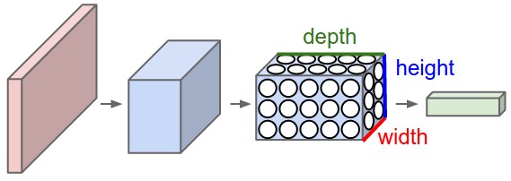
A simple CNN is a sequence of layers, and every layer of a CNN transforms one volume of activations to another through a differentiable function. We use three main types of layers to build CNN architectures: Convolutional Layer, Pooling Layer, and Fully-Connected Layer (exactly as seen in regular Neural Networks). We will stack these layers to form a full CNN architecture.
A simple CNN for image classification could have the architecture:
CNNs transform the original image layer by layer from the original pixel values to the final class scores.
Observe that some layers contain parameters and other don’t. In particular, the CNN layers perform transformations that are a function of not only the activations in the input volume, but also of the parameters (the weights and biases of the neurons). On the other hand, the RELU/POOL layers will implement a fixed function. The parameters in the CONV/FC layers will be trained with gradient descent so that the class scores that the CNN computes are consistent with the labels in the training set for each image.
In summary:
As discussed above, CNNs are neural networks built from the assumption that the inputs to the network are 2D images. This is important because the number of features or pixels in images grows very fast with the image size, and an enormous number of weights and biases are needed in order to build an accurate network.
As before, we still have our input, a hidden layer and an output. What's novel about convolutional networks are the convolutional and pooling layers stacked in pairs between the input and the hidden layer. In addition, the data is no longer represented as a 2D feature matrix, instead each input is a number of 2D matrices, typically 1 for each color dimension (Red, Green, Blue).
It means that to represent the entire dataset of images, we require a 4D matrix or tensor. This tensor has the dimensions: $$ (n_{inputs},\, n_{pixels, width},\, n_{pixels, height},\, depth) . $$
The MNIST dataset consists of grayscale images with a pixel size of \( 28\times 28 \), meaning we require \( 28 \times 28 = 724 \) weights to each neuron in the first hidden layer.
If we were to analyze images of size \( 128\times 128 \) we would require \( 128 \times 128 = 16384 \) weights to each neuron. Even worse if we were dealing with color images, as most images are, we have an image matrix of size \( 128\times 128 \) for each color dimension (Red, Green, Blue), meaning 3 times the number of weights \( = 49152 \) are required for every single neuron in the first hidden layer.
Therefore, instead of connecting every single pixel to a neuron in the first hidden layer, as we have previously done with deep neural networks, we can instead connect each neuron to a small part of the image (in all 3 RGB depth dimensions). The size of each small area is fixed, and known as a receptive.
A convolution is performed on the image which outputs a 3D volume of neurons. The weights to the input are arranged in a number of 2D matrices, known as filters.
Each filter slides along the input image, taking the dot product between each small part of the image and the filter, in all depth dimensions. This is then passed through a non-linear function, typically the Rectified Linear (ReLu) function, which serves as the activation of the neurons in the first convolutional layer. This is further passed through a pooling layer, which reduces the size of the convolutional layer, e.g. by taking the maximum or average across some small regions, and this serves as input to the next convolutional layer.
By systematically reducing the size of the input volume, through convolution and pooling, the network should create representations of small parts of the input, and then from them assemble representations of larger areas. The final pooling layer is flattened to serve as input to a hidden layer, such that each neuron in the final pooling layer is connected to every single neuron in the hidden layer. This then serves as input to the output layer, e.g. a softmax output for classification.
# import necessary packages
import numpy as np
import matplotlib.pyplot as plt
from sklearn import datasets


# ensure the same random numbers appear every time
np.random.seed(0)

# display images in notebook
%matplotlib inline
plt.rcParams['figure.figsize'] = (12,12)


# download MNIST dataset
digits = datasets.load_digits()

# define inputs and labels
inputs = digits.images
labels = digits.target

# RGB images have a depth of 3
# our images are grayscale so they should have a depth of 1
inputs = inputs[:,:,:,np.newaxis]

print("inputs = (n_inputs, pixel_width, pixel_height, depth) = " + str(inputs.shape))
print("labels = (n_inputs) = " + str(labels.shape))


# choose some random images to display
n_inputs = len(inputs)
indices = np.arange(n_inputs)
random_indices = np.random.choice(indices, size=5)

for i, image in enumerate(digits.images[random_indices]):
    plt.subplot(1, 5, i+1)
    plt.axis('off')
    plt.imshow(image, cmap=plt.cm.gray_r, interpolation='nearest')
    plt.title("Label: %d" % digits.target[random_indices[i]])
plt.show()
from keras.utils import to_categorical
from sklearn.model_selection import train_test_split

# representation of labels
labels = to_categorical(labels)

# split into train and test data
# one-liner from scikit-learn library
train_size = 0.8
test_size = 1 - train_size
X_train, X_test, Y_train, Y_test = train_test_split(inputs, labels, train_size=train_size,
                                                    test_size=test_size)
We need to define model and architecture and choose cost function and optmizer.
import tensorflow as tf

class ConvolutionalNeuralNetworkTensorflow:
    def __init__(
        self,
        X_train,
        Y_train,
        X_test,
        Y_test,
        n_filters=10,
        n_neurons_connected=50,
        n_categories=10,
        receptive_field=3,
        stride=1,
        padding=1,
        epochs=10,
        batch_size=100,
        eta=0.1,
        lmbd=0.0,
    ):

        self.global_step = tf.Variable(0, dtype=tf.int32, trainable=False, name='global_step')

        self.X_train = X_train
        self.Y_train = Y_train
        self.X_test = X_test
        self.Y_test = Y_test

        self.n_inputs, self.input_width, self.input_height, self.depth = X_train.shape

        self.n_filters = n_filters
        self.n_downsampled = int(self.input_width*self.input_height*n_filters / 4)
        self.n_neurons_connected = n_neurons_connected
        self.n_categories = n_categories

        self.receptive_field = receptive_field
        self.stride = stride
        self.strides = [stride, stride, stride, stride]
        self.padding = padding

        self.epochs = epochs
        self.batch_size = batch_size
        self.iterations = self.n_inputs // self.batch_size
        self.eta = eta
        self.lmbd = lmbd

        self.create_placeholders()
        self.create_CNN()
        self.create_loss()
        self.create_optimiser()
        self.create_accuracy()

    def create_placeholders(self):
        with tf.name_scope('data'):
            self.X = tf.placeholder(tf.float32, shape=(None, self.input_width, self.input_height, self.depth), name='X_data')
            self.Y = tf.placeholder(tf.float32, shape=(None, self.n_categories), name='Y_data')

    def create_CNN(self):
        with tf.name_scope('CNN'):

            # Convolutional layer
            self.W_conv = self.weight_variable([self.receptive_field, self.receptive_field, self.depth, self.n_filters], name='conv', dtype=tf.float32)
            b_conv = self.weight_variable([self.n_filters], name='conv', dtype=tf.float32)
            z_conv = tf.nn.conv2d(self.X, self.W_conv, self.strides, padding='SAME', name='conv') + b_conv
            a_conv = tf.nn.relu(z_conv)

            # 2x2 max pooling
            a_pool = tf.nn.max_pool(a_conv, [1, 2, 2, 1], [1, 2, 2, 1], padding='SAME', name='pool')

            # Fully connected layer
            a_pool_flat = tf.reshape(a_pool, [-1, self.n_downsampled])
            self.W_fc = self.weight_variable([self.n_downsampled, self.n_neurons_connected], name='fc', dtype=tf.float32)
            b_fc = self.bias_variable([self.n_neurons_connected], name='fc', dtype=tf.float32)
            a_fc = tf.nn.relu(tf.matmul(a_pool_flat, self.W_fc) + b_fc)

            # Output layer
            self.W_out = self.weight_variable([self.n_neurons_connected, self.n_categories], name='out', dtype=tf.float32)
            b_out = self.bias_variable([self.n_categories], name='out', dtype=tf.float32)
            self.z_out = tf.matmul(a_fc, self.W_out) + b_out

    def create_loss(self):
        with tf.name_scope('loss'):
            softmax_loss = tf.reduce_mean(tf.nn.softmax_cross_entropy_with_logits_v2(labels=self.Y, logits=self.z_out))

            regularizer_loss_conv = tf.nn.l2_loss(self.W_conv)
            regularizer_loss_fc = tf.nn.l2_loss(self.W_fc)
            regularizer_loss_out = tf.nn.l2_loss(self.W_out)
            regularizer_loss = self.lmbd*(regularizer_loss_conv + regularizer_loss_fc + regularizer_loss_out)

            self.loss = softmax_loss + regularizer_loss

    def create_accuracy(self):
        with tf.name_scope('accuracy'):
            probabilities = tf.nn.softmax(self.z_out)
            predictions = tf.argmax(probabilities, 1)
            labels = tf.argmax(self.Y, 1)

            correct_predictions = tf.equal(predictions, labels)
            correct_predictions = tf.cast(correct_predictions, tf.float32)
            self.accuracy = tf.reduce_mean(correct_predictions)

    def create_optimiser(self):
        with tf.name_scope('optimizer'):
            self.optimizer = tf.train.GradientDescentOptimizer(learning_rate=self.eta).minimize(self.loss, global_step=self.global_step)

    def weight_variable(self, shape, name='', dtype=tf.float32):
        initial = tf.truncated_normal(shape, stddev=0.1)
        return tf.Variable(initial, name=name, dtype=dtype)

    def bias_variable(self, shape, name='', dtype=tf.float32):
        initial = tf.constant(0.1, shape=shape)
        return tf.Variable(initial, name=name, dtype=dtype)

    def fit(self):
        data_indices = np.arange(self.n_inputs)

        with tf.Session() as sess:
            sess.run(tf.global_variables_initializer())
            for i in range(self.epochs):
                for j in range(self.iterations):
                    chosen_datapoints = np.random.choice(data_indices, size=self.batch_size, replace=False)
                    batch_X, batch_Y = self.X_train[chosen_datapoints], self.Y_train[chosen_datapoints]

                    sess.run([CNN.loss, CNN.optimizer],
                        feed_dict={CNN.X: batch_X,
                                   CNN.Y: batch_Y})
                    accuracy = sess.run(CNN.accuracy,
                        feed_dict={CNN.X: batch_X,
                                   CNN.Y: batch_Y})
                    step = sess.run(CNN.global_step)

            self.train_loss, self.train_accuracy = sess.run([CNN.loss, CNN.accuracy],
                feed_dict={CNN.X: self.X_train,
                           CNN.Y: self.Y_train})

            self.test_loss, self.test_accuracy = sess.run([CNN.loss, CNN.accuracy],
                feed_dict={CNN.X: self.X_test,
                           CNN.Y: self.Y_test})
We need now to train the model, evaluate it and test its performance on test data, and eventually include hyperparameters.
epochs = 100
batch_size = 100
n_filters = 10
n_neurons_connected = 50
n_categories = 10

eta_vals = np.logspace(-5, 1, 7)
lmbd_vals = np.logspace(-5, 1, 7)
CNN_tf = np.zeros((len(eta_vals), len(lmbd_vals)), dtype=object)

for i, eta in enumerate(eta_vals):
    for j, lmbd in enumerate(lmbd_vals):
        CNN = ConvolutionalNeuralNetworkTensorflow(X_train, Y_train, X_test, Y_test,
                                      n_filters=n_filters, n_neurons_connected=n_neurons_connected,
                                      n_categories=n_categories, epochs=epochs, batch_size=batch_size,
                                      eta=eta, lmbd=lmbd)
        CNN.fit()

        print("Learning rate = ", eta)
        print("Lambda = ", lmbd)
        print("Test accuracy: %.3f" % CNN.test_accuracy)
        print()

        CNN_tf[i][j] = CNN
# visual representation of grid search
# uses seaborn heatmap, could probably do this in matplotlib
import seaborn as sns

sns.set()

train_accuracy = np.zeros((len(eta_vals), len(lmbd_vals)))
test_accuracy = np.zeros((len(eta_vals), len(lmbd_vals)))

for i in range(len(eta_vals)):
    for j in range(len(lmbd_vals)):
        CNN = CNN_tf[i][j]

        train_accuracy[i][j] = CNN.train_accuracy
        test_accuracy[i][j] = CNN.test_accuracy


fig, ax = plt.subplots(figsize = (10, 10))
sns.heatmap(train_accuracy, annot=True, ax=ax, cmap="viridis")
ax.set_title("Training Accuracy")
ax.set_ylabel("$\eta$")
ax.set_xlabel("$\lambda$")
plt.show()

fig, ax = plt.subplots(figsize = (10, 10))
sns.heatmap(test_accuracy, annot=True, ax=ax, cmap="viridis")
ax.set_title("Test Accuracy")
ax.set_ylabel("$\eta$")
ax.set_xlabel("$\lambda$")
plt.show()
from keras.models import Sequential
from keras.layers.convolutional import Conv2D
from keras.layers.convolutional import MaxPooling2D
from keras.layers import Flatten
from keras.layers import Dense
from keras.regularizers import l2
from keras.optimizers import SGD

def create_convolutional_neural_network_keras(input_shape, receptive_field,
                                              n_filters, n_neurons_connected, n_categories,
                                              eta, lmbd):
    model = Sequential()
    model.add(Conv2D(n_filters, (receptive_field, receptive_field), input_shape=input_shape, padding='same',
              activation='relu', kernel_regularizer=l2(lmbd)))
    model.add(MaxPooling2D(pool_size=(2, 2)))
    model.add(Flatten())
    model.add(Dense(n_neurons_connected, activation='relu', kernel_regularizer=l2(lmbd)))
    model.add(Dense(n_categories, activation='softmax', kernel_regularizer=l2(lmbd)))

    sgd = SGD(lr=eta)
    model.compile(loss='categorical_crossentropy', optimizer=sgd, metrics=['accuracy'])

    return model

epochs = 100
batch_size = 100
input_shape = X_train.shape[1:4]
receptive_field = 3
n_filters = 10
n_neurons_connected = 50
n_categories = 10

eta_vals = np.logspace(-5, 1, 7)
lmbd_vals = np.logspace(-5, 1, 7)
CNN_keras = np.zeros((len(eta_vals), len(lmbd_vals)), dtype=object)

for i, eta in enumerate(eta_vals):
    for j, lmbd in enumerate(lmbd_vals):
        CNN = create_convolutional_neural_network_keras(input_shape, receptive_field,
                                              n_filters, n_neurons_connected, n_categories,
                                              eta, lmbd)
        CNN.fit(X_train, Y_train, epochs=epochs, batch_size=batch_size, verbose=0)
        scores = CNN.evaluate(X_test, Y_test)

        CNN_keras[i][j] = CNN

        print("Learning rate = ", eta)
        print("Lambda = ", lmbd)
        print("Test accuracy: %.3f" % scores[1])
        print()
# visual representation of grid search
# uses seaborn heatmap, could probably do this in matplotlib
import seaborn as sns

sns.set()

train_accuracy = np.zeros((len(eta_vals), len(lmbd_vals)))
test_accuracy = np.zeros((len(eta_vals), len(lmbd_vals)))

for i in range(len(eta_vals)):
    for j in range(len(lmbd_vals)):
        CNN = CNN_keras[i][j]

        train_accuracy[i][j] = CNN.evaluate(X_train, Y_train)[1]
        test_accuracy[i][j] = CNN.evaluate(X_test, Y_test)[1]


fig, ax = plt.subplots(figsize = (10, 10))
sns.heatmap(train_accuracy, annot=True, ax=ax, cmap="viridis")
ax.set_title("Training Accuracy")
ax.set_ylabel("$\eta$")
ax.set_xlabel("$\lambda$")
plt.show()

fig, ax = plt.subplots(figsize = (10, 10))
sns.heatmap(test_accuracy, annot=True, ax=ax, cmap="viridis")
ax.set_title("Test Accuracy")
ax.set_ylabel("$\eta$")
ax.set_xlabel("$\lambda$")
plt.show()
We end our discussion on neural networks with a discussion on how to solve differential equations. Here we focus first on the classical exponential decay in one dimension. Thereafter we switch to the Poisson equation in one dimension.
The aim is to see if we can use a neural network to solve $$ \begin{equation} \label{eq:ode} g'(x) = -\gamma g(x) \end{equation} $$
where \( g(0) = g_0 \) with \( \gamma \) and \( g_0 \) being some chosen values. This equation is an ordinary differential equation since the function we have to solve for, \( g(x) \), is of one variable.
Here we set \( \gamma = 2 \) and \( g_0 = 10 \) but feel free to change them and see how the neural network performs.
To begin with, a trial solution \( g_t(t) \) must be chosen. A general trial solution for ordinary differential equations could be $$ g_t(x, P) = h_1(x) + h_2(x, N(x, P)), $$
with \( h_1(x) \) ensuring that \( g_t(x) \) satisfies some conditions and \( h_2(x,N(x, P)) \) an expression involving \( x \) and the output from the neural network \( N(x,P) \) with \( P \) being the collection of the weights and biases for each layer.
It is assumed that there are no weights and bias at the input layer, so \( P = \{ P_{\mathrm{hidden}}, P_{\mathrm{output}} \} \). If there are \( N_{\mathrm{hidden} } \) neurons in the hidden layer, then \( P_{\mathrm{hidden}} \) is an \( N_{\mathrm{hidden} } \times 2 \) matrix.
The first column in \( P_{\mathrm{hidden} } \) represents the bias for each neuron in the hidden layer and the second column represents the weigths for each neuron. If there are \( N_{\mathrm{output} } \) neurons in the output layer, then \( P_{\mathrm{output}} \) is a \( N_{\mathrm{output} } \times (1 + N_{\mathrm{hidden} }) \) matrix. Its first column represents the bias of each neuron and the remaining columns represents the weights to each neuron.
We have \( g(0) = g_0 \). The trial solution must fulfill this condition to be a proper solution of \eqref{eq:ode}.
A possible way to ensure that \( g_t(0, P) = g_0 \), is to let \( F(N(x,P)) = x\cdot N(x,P) \) and \( A(x) = g_0 \). This gives the following trial solution: $$ \begin{equation} g_t(x, P) = g_0 + x \cdot N(x, P). \label{_auto11} \end{equation} $$
Often, the role of a neural network is to minimize its parameters with respect to some given error criteria. This criteria, the cost or loss function, is a measure of how much error the output of the network has compared to some given known answers. A reformulation of \eqref{eq:ode} must therefore be done, such that it describes the problem a neural network can solve.
The neural network must find the set of weigths and biases \( P \) such that the trial solution in satisfies \eqref{eq:ode}. The trial solution has been chosen such that it already solves the condition \( g(0) = g_0 \). What remains, is to find \( P \) such that $$ \begin{equation} g_t'(x, P) = - \gamma g_t(x, P) \label{_auto12} \end{equation} $$
is fulfilled as best as possible.
Having two sides of an equation as equal as possible, means that the absolute or squared difference between the sides must be as close to zero as small. In this case, the difference squared is an appropiate measurement of how errorneous the trial solution is with respect to \( P \) of the neural network. Therefore, the problem our network must solve, is $$ \min_{P}\Big\{ \big(g_t'(x, P) - ( -\gamma g_t(x, P) \big)^2 \Big\} $$
or, in terms of weights and biases for each layer: $$ \min_{P_{\mathrm{hidden} }, \ P_{\mathrm{output} }}\Big\{ \big(g_t'(x, \{ P_{\mathrm{hidden} }, P_{\mathrm{output} }\}) - ( -\gamma g_t(x, \{ P_{\mathrm{hidden} }, P_{\mathrm{output} }\}) \big)^2 \Big\} $$
for an input value \( x \). If the neural network evaluates \( g_t(x, P) \) at more avalues for \( x \), say \( N \) values \( x_i \) for \( i = 1, \dots, N \), then the total error to minimize is $$ \begin{equation} \label{eq:min} \min_{P}\Big\{\sum_i \big(g_t'(x_i, P) - ( -\gamma g_t(x_i, P) \big)^2 \Big\} \end{equation} $$
Letting \( c(x, P) = \sum_i \big(g_t'(x_i, P) - ( -\gamma g_t(x_i, P) \big)^2 \) denote the cost function, the minimization problem of which our network must solve, is $$ \min_{P} c(x, P) $$
or in terms of \( P_{\mathrm{hidden} } \) and \( P_{\mathrm{output} } \) $$ \min_{P_{\mathrm{hidden} }, \ P_{\mathrm{output} }} c(x, \{P_{\mathrm{hidden} }, P_{\mathrm{output} }\}) $$
The next step is to decide how the neural net \( N(x, P) \) should be. In this case, the neural network is made from scratch to understand better how a neural network works, gain more control over its architecture, and see how Autograd can be used to simplify the implementation.
Since a deep neural network (DNN) is a neural network with more than one hidden layer, we can first look on how to implement a neural network. Having an implementation of a neural network at hand, an extension of it into a deep neural network would (hopefully) be painless.
For simplicity, we assume that the input is an array \( \hat{x}= (x_1, \dots, x_N) \) with \( N \) elements. It is at these points the neural network should find \( P \) such that it fulfills \eqref{eq:min}. All the ingredients discussed earlier, from the activation function, hidden layers and their weights, biases etc are included below.
# Note that we use the  numpy wrapper for Autograd (see the gradient descent  slides)
import autograd.numpy as np
from autograd import grad, elementwise_grad
import autograd.numpy.random as npr
from matplotlib import pyplot as plt

def sigmoid(z):
    return 1/(1 + np.exp(-z))

def neural_network(params, x):

    # Find the weights (including and biases) for the hidden and output layer.
    # Assume that params is a list of parameters for each layer.
    # The biases are the first element for each array in params,
    # and the weights are the remaning elements in each array in params.

    w_hidden = params[0]
    w_output = params[1]

    # Assumes input x being an one-dimensional array
    num_values = np.size(x)
    x = x.reshape(-1, num_values)

    # Assume that the input layer does nothing to the input x
    x_input = x

    ## Hidden layer:

    # Add a row of ones to include bias
    x_input = np.concatenate((np.ones((1,num_values)), x_input ), axis = 0)

    z_hidden = np.matmul(w_hidden, x_input)
    x_hidden = sigmoid(z_hidden)

    ## Output layer:

    # Include bias:
    x_hidden = np.concatenate((np.ones((1,num_values)), x_hidden ), axis = 0)

    z_output = np.matmul(w_output, x_hidden)
    x_output = z_output

    return x_output
Now that the feedforward can be done, the next step is to decide how the parameters should change such that they minimize the cost function.
Recall that the chosen cost function for this problem is $$ c(x, P) = \sum_i \big(g_t'(x_i, P) - ( -\gamma g_t(x_i, P) \big)^2 $$
In order to minimize it, an optimization method must be chosen.
Here, gradient descent with a constant step size has been chosen.
Before looking at the gradient descent method, let us set up the cost function along with the right ride of the ODE and trial solution.
# The trial solution using the deep neural network:
def g_trial(x,params, g0 = 10):
    return g0 + x*neural_network(params,x)

# The right side of the ODE:
def g(x, g_trial, gamma = 2):
    return -gamma*g_trial

# The cost function:
def cost_function(P, x):

    # Evaluate the trial function with the current parameters P
    g_t = g_trial(x,P)

    # Find the derivative w.r.t x of the neural network
    d_net_out = elementwise_grad(neural_network,1)(P,x)

    # Find the derivative w.r.t x of the trial function
    d_g_t = elementwise_grad(g_trial,0)(x,P)

    # The right side of the ODE
    func = g(x, g_t)

    err_sqr = (d_g_t - func)**2
    cost_sum = np.sum(err_sqr)

    return cost_sum
The idea of the gradient descent algorithm is to update parameters in direction where the cost function decreases goes to a minimum.
In general, the update of some parameters \( \hat{\omega} \) given a cost function defined by some weights \( \hat{\omega} \), \( c(x, \hat{\omega}) \), goes as follows: $$ \hat{\omega}_{\mathrm{new} } = \hat{\omega} - \lambda \nabla_{\hat{\omega}} c(x, \hat{\omega}), $$
for a number of iterations or until \( \big|\big| \hat{\omega}_{\mathrm{new} } - \hat{\omega} \big|\big| \) is smaller than some given tolerance.
The value of \( \lambda \) decides how large steps the algorithm must take in the direction of $ \nabla_{\hat{\omega}} c(x, \hat{\omega})$. The notatation \( \nabla_{\hat{\omega}} \) denotes the gradient with respect to the elements in \( \hat{\omega} \).
In our case, we have to minimize the cost function \( c(x, P) \) with respect to the two sets of weights and bisases, that is for the hidden layer \( P_{\mathrm{hidden} } \) and for the ouput layer \( P_{\mathrm{output} } \) .
This means that \( P_{\mathrm{hidden} } \) and \( P_{\mathrm{output} } \) is updated by $$ \begin{align} P_{\mathrm{hidden},\mathrm{new}} &= P_{\mathrm{hidden}} - \lambda \nabla_{P_{\mathrm{hidden}}} c(x, P) \label{_auto13}\\ P_{\mathrm{output},\mathrm{new}} &= P_{\mathrm{output}} - \lambda \nabla_{P_{\mathrm{output}}} c(x, P) \label{_auto14} \end{align} $$
This might look like a cumberstone to set up the correct expression for finding the gradients. Luckily, Autograd comes to the rescue.
def solve_ode_neural_network(x, num_neurons_hidden, num_iter, lmb):
    ## Set up initial weigths and biases

    # For the hidden layer
    p0 = npr.randn(num_neurons_hidden, 2 )

    # For the output layer
    p1 = npr.randn(1, num_neurons_hidden + 1 ) # +1 since bias is included

    P = [p0, p1]

    print('Initial cost: %g'%cost_function(P, x))

    ## Start finding the optimal weigths using gradient descent

    # Find the Python function that represents the gradient of the cost function
    # w.r.t the 0-th input argument -- that is the weights and biases in the hidden and output layer
    cost_function_grad = grad(cost_function,0)

    # Let the update be done num_iter times
    for i in range(num_iter):
        # Evaluate the gradient at the current weights and biases in P.
        # The cost_grad consist now of two arrays;
        # one for the gradient w.r.t P_hidden and
        # one for the gradient w.r.t P_output
        cost_grad =  cost_function_grad(P, x)

        P[0] = P[0] - lmb * cost_grad[0]
        P[1] = P[1] - lmb * cost_grad[1]

    print('Final cost: %g'%cost_function(P, x))

    return P
As previously stated, a Deep Neural Network (DNN) follows the same concept of a neural network, but having more than one hidden layer. Suppose that the network has \( N_{\mathrm{hidden}} \) hidden layers where the \( l \)-th layer has \( N_{\mathrm{hidden}}^{(l)} \) neurons. The input is still assumed to be an array of size \( 1 \times N \). The network must now try to optimalize its output with respect to the collection of weigths and biases \( P = \big\{P_{\mathrm{input} }, \ P_{\mathrm{hidden} }^{(1)}, \ P_{\mathrm{hidden} }^{(2)}, \ \dots , \ P_{\mathrm{hidden} }^{(N_{\mathrm{hidden}})}, \ P_{\mathrm{output} }\big\} \).
def deep_neural_network(deep_params, x):
    # N_hidden is the number of hidden layers
    N_hidden = np.size(deep_params) - 1 # -1 since params consist of parameters to all the hidden layers AND the output layer

    # Assumes input x being an one-dimensional array
    num_values = np.size(x)
    x = x.reshape(-1, num_values)

    # Assume that the input layer does nothing to the input x
    x_input = x

    # Due to multiple hidden layers, define a variable referencing to the
    # output of the previous layer:
    x_prev = x_input

    ## Hidden layers:

    for l in range(N_hidden):
        # From the list of parameters P; find the correct weigths and bias for this layer
        w_hidden = deep_params[l]

        # Add a row of ones to include bias
        x_prev = np.concatenate((np.ones((1,num_values)), x_prev ), axis = 0)

        z_hidden = np.matmul(w_hidden, x_prev)
        x_hidden = sigmoid(z_hidden)

        # Update x_prev such that next layer can use the output from this layer
        x_prev = x_hidden

    ## Output layer:

    # Get the weights and bias for this layer
    w_output = deep_params[-1]

    # Include bias:
    x_prev = np.concatenate((np.ones((1,num_values)), x_prev), axis = 0)

    z_output = np.matmul(w_output, x_prev)
    x_output = z_output

    return x_output
This step is very similar for the neural network. The idea in this step is the same as for the neural network, but with more parameters to update for. Again there is no need for computing the gradients analytically since Autograd does the work for us.
# The trial solution using the deep neural network:
def g_trial_deep(x,params, g0 = 10):
    return g0 + x*deep_neural_network(params,x)

# The same cost function as for the neural network, but calls deep_neural_network instead.
def cost_function_deep(P, x):

    # Evaluate the trial function with the current parameters P
    g_t = g_trial_deep(x,P)

    # Find the derivative w.r.t x of the neural network
    d_net_out = elementwise_grad(deep_neural_network,1)(P,x)

    # Find the derivative w.r.t x of the trial function
    d_g_t = elementwise_grad(g_trial_deep,0)(x,P)

    # The right side of the ODE
    func = g(x, g_t)

    err_sqr = (d_g_t - func)**2
    cost_sum = np.sum(err_sqr)

    return cost_sum

def solve_ode_deep_neural_network(x, num_neurons, num_iter, lmb):
    # num_hidden_neurons is now a list of number of neurons within each hidden layer

    # Find the number of hidden layers:
    N_hidden = np.size(num_neurons)

    ## Set up initial weigths and biases

    # Initialize the list of parameters:
    P = [None]*(N_hidden + 1) # + 1 to include the output layer

    P[0] = npr.randn(num_neurons[0], 2 )
    for l in range(1,N_hidden):
        P[l] = npr.randn(num_neurons[l], num_neurons[l-1] + 1) # +1 to include bias

    # For the output layer
    P[-1] = npr.randn(1, num_neurons[-1] + 1 ) # +1 since bias is included

    print('Initial cost: %g'%cost_function_deep(P, x))

    ## Start finding the optimal weigths using gradient descent

    # Find the Python function that represents the gradient of the cost function
    # w.r.t the 0-th input argument -- that is the weights and biases in the hidden and output layer
    cost_function_deep_grad = grad(cost_function_deep,0)

    # Let the update be done num_iter times
    for i in range(num_iter):
        # Evaluate the gradient at the current weights and biases in P.
        # The cost_grad consist now of N_hidden + 1 arrays; the gradient w.r.t the weights and biases
        # in the hidden layers and output layers evaluated at x.
        cost_deep_grad =  cost_function_deep_grad(P, x)

        for l in range(N_hidden+1):
            P[l] = P[l] - lmb * cost_deep_grad[l]

    print('Final cost: %g'%cost_function_deep(P, x))

    return P
Finally, having set up the networks we are ready to use them to solve the ODE problem. We add the analytical solution
def g_analytic(x, gamma = 2, g0 = 10):
    return g0*np.exp(-gamma*x)
The code below solves the ODE using a neural network. The number of values for the input \( \vec x \) is 10, number of hidden neurons in the hidden layer being 10 and th step size used in gradien descent \( \lambda = 0.001 \). The program updates the weights and biases in the network for a given number of iterations. Finally, it plots the results from using the neural network along with the analytical solution.
npr.seed(15)

## Decide the vales of arguments to the function to solve
N = 10
x = np.linspace(0, 1, N)

## Set up the initial parameters
num_hidden_neurons = 10
num_iter = 10000
lmb = 0.001

P = solve_ode_neural_network(x, num_hidden_neurons, num_iter, lmb)

res = g_trial(x,P)
res_analytical = g_analytic(x)

print('Max absolute difference: %g'%np.max(np.abs(res - res_analytical)))

plt.figure(figsize=(10,10))

plt.title('Performance of neural network solving an ODE compared to the analytical solution')
plt.plot(x, res_analytical)
plt.plot(x, res[0,:])
plt.legend(['analytical','nn'])
plt.xlabel('x')
plt.ylabel('g(x)')
plt.show()
npr.seed(15)

## Decide the vales of arguments to the function to solve
N = 10
x = np.linspace(0, 1, N)

## Set up the initial parameters
num_hidden_neurons = np.array([10,10])
num_iter = 10000
lmb = 0.001

P = solve_ode_deep_neural_network(x, num_hidden_neurons, num_iter, lmb)

res = g_trial_deep(x,P)
res_analytical = g_analytic(x)

plt.figure(figsize=(10,10))

plt.title('Performance of a deep neural network solving an ODE compared to the analytical solution')
plt.plot(x, res_analytical)
plt.plot(x, res[0,:])
plt.legend(['analytical','dnn'])
plt.ylabel('g(x)')
plt.show()
By rewriting the ODE as a minimization problem, it was possible to solve equation using either a neural network (one hidden layer) or a deep neural network (more than one hidden layers). How well the network performed is measured by a specified cost function, which is the function the network tries to minimize. Using a trial solution which satisfies the additional condition and being defined by using the output from the network in some way, the minimization problem could be explicitly defined for out network to solve. The proposed solution from the network is then the trial solution with parameters, that is weights and biases within each layer in the network, such that the solution minimizes the cost function.