
5. Resampling Methods
5.1. Introduction
Resampling methods are an indispensable tool in modern statistics. They involve repeatedly drawing samples from a training set and refitting a model of interest on each sample in order to obtain additional information about the fitted model. For example, in order to estimate the variability of a linear regression fit, we can repeatedly draw different samples from the training data, fit a linear regression to each new sample, and then examine the extent to which the resulting fits differ. Such an approach may allow us to obtain information that would not be available from fitting the model only once using the original training sample.
Two resampling methods are often used in Machine Learning analyses,
The bootstrap method
and Cross-Validation
In addition there are several other methods such as the Jackknife and the Blocking methods. We will discuss in particular cross-validation and the bootstrap method.
Resampling approaches can be computationally expensive, because they involve fitting the same statistical method multiple times using different subsets of the training data. However, due to recent advances in computing power, the computational requirements of resampling methods generally are not prohibitive. In this chapter, we discuss two of the most commonly used resampling methods, cross-validation and the bootstrap. Both methods are important tools in the practical application of many statistical learning procedures. For example, cross-validation can be used to estimate the test error associated with a given statistical learning method in order to evaluate its performance, or to select the appropriate level of flexibility. The process of evaluating a model’s performance is known as model assessment, whereas the process of selecting the proper level of flexibility for a model is known as model selection. The bootstrap is widely used.
Our simulations can be treated as computer experiments. This is particularly the case for Monte Carlo methods
The results can be analysed with the same statistical tools as we would use analysing experimental data.
As in all experiments, we are looking for expectation values and an estimate of how accurate they are, i.e., possible sources for errors.
5.2. Reminder on Statistics
As in other experiments, many numerical experiments have two classes of errors:
Statistical errors
Systematical errors
Statistical errors can be estimated using standard tools from statistics
Systematical errors are method specific and must be treated differently from case to case.
The
advantage of doing linear regression is that we actually end up with
analytical expressions for several statistical quantities.
Standard least squares and Ridge regression allow us to
derive quantities like the variance and other expectation values in a
rather straightforward way.
It is assumed that \(\varepsilon_i \sim \mathcal{N}(0, \sigma^2)\) and the \(\varepsilon_{i}\) are independent, i.e.:
The randomness of \(\varepsilon_i\) implies that \(\mathbf{y}_i\) is also a random variable. In particular, \(\mathbf{y}_i\) is normally distributed, because \(\varepsilon_i \sim \mathcal{N}(0, \sigma^2)\) and \(\mathbf{X}_{i,\ast} \, \boldsymbol{\beta}\) is a non-random scalar. To specify the parameters of the distribution of \(\mathbf{y}_i\) we need to calculate its first two moments.
Recall that \(\boldsymbol{X}\) is a matrix of dimensionality \(n\times p\). The notation above \(\mathbf{X}_{i,\ast}\) means that we are looking at the row number \(i\) and perform a sum over all values \(p\).
The assumption we have made here can be summarized as (and this is going to be useful when we discuss the bias-variance trade off) that there exists a function \(f(\boldsymbol{x})\) and a normal distributed error \(\boldsymbol{\varepsilon}\sim \mathcal{N}(0, \sigma^2)\) which describe our data
We approximate this function with our model from the solution of the linear regression equations, that is our function \(f\) is approximated by \(\boldsymbol{\tilde{y}}\) where we want to minimize \((\boldsymbol{y}-\boldsymbol{\tilde{y}})^2\), our MSE, with
We can calculate the expectation value of \(\boldsymbol{y}\) for a given element \(i\)
while its variance is
Hence, \(y_i \sim \mathcal{N}( \mathbf{X}_{i, \ast} \, \boldsymbol{\beta}, \sigma^2)\), that is \(\boldsymbol{y}\) follows a normal distribution with mean value \(\boldsymbol{X}\boldsymbol{\beta}\) and variance \(\sigma^2\) (not be confused with the singular values of the SVD).
With the OLS expressions for the parameters \(\boldsymbol{\beta}\) we can evaluate the expectation value
This means that the estimator of the regression parameters is unbiased.
We can also calculate the variance
The variance of \(\boldsymbol{\beta}\) is
where we have used that \(\mathbb{E} (\mathbf{Y} \mathbf{Y}^{T}) = \mathbf{X} \, \boldsymbol{\beta} \, \boldsymbol{\beta}^{T} \, \mathbf{X}^{T} + \sigma^2 \, \mathbf{I}_{nn}\). From \(\mbox{Var}(\boldsymbol{\beta}) = \sigma^2 \, (\mathbf{X}^{T} \mathbf{X})^{-1}\), one obtains an estimate of the variance of the estimate of the \(j\)-th regression coefficient: \(\boldsymbol{\sigma}^2 (\boldsymbol{\beta}_j ) = \boldsymbol{\sigma}^2 \sqrt{ [(\mathbf{X}^{T} \mathbf{X})^{-1}]_{jj} }\). This may be used to construct a confidence interval for the estimates.
In a similar way, we can obtain analytical expressions for say the expectation values of the parameters \(\boldsymbol{\beta}\) and their variance when we employ Ridge regression, allowing us again to define a confidence interval.
It is rather straightforward to show that
We see clearly that \(\mathbb{E} \big[ \boldsymbol{\beta}^{\mathrm{Ridge}} \big] \not= \boldsymbol{\beta}^{\mathrm{OLS}}\) for any \(\lambda > 0\). We say then that the ridge estimator is biased.
We can also compute the variance as
and it is easy to see that if the parameter \(\lambda\) goes to infinity then the variance of Ridge parameters \(\boldsymbol{\beta}\) goes to zero.
With this, we can compute the difference
The difference is non-negative definite since each component of the matrix product is non-negative definite. This means the variance we obtain with the standard OLS will always for \(\lambda > 0\) be larger than the variance of \(\boldsymbol{\beta}\) obtained with the Ridge estimator. This has interesting consequences when we discuss the so-called bias-variance trade-off below.
5.3. Resampling methods
With all these analytical equations for both the OLS and Ridge regression, we will now outline how to assess a given model. This will lead us to a discussion of the so-called bias-variance tradeoff (see below) and so-called resampling methods.
One of the quantities we have discussed as a way to measure errors is the mean-squared error (MSE), mainly used for fitting of continuous functions. Another choice is the absolute error.
In the discussions below we will focus on the MSE and in particular since we will split the data into test and training data, we discuss the
prediction error or simply the test error \(\mathrm{Err_{Test}}\), where we have a fixed training set and the test error is the MSE arising from the data reserved for testing. We discuss also the
training error \(\mathrm{Err_{Train}}\), which is the average loss over the training data.
As our model becomes more and more complex, more of the training data tends to used. The training may thence adapt to more complicated structures in the data. This may lead to a decrease in the bias (see below for code example) and a slight increase of the variance for the test error. For a certain level of complexity the test error will reach minimum, before starting to increase again. The training error reaches a saturation.
Two famous resampling methods are the independent bootstrap and the jackknife.
The jackknife is a special case of the independent bootstrap. Still, the jackknife was made popular prior to the independent bootstrap. And as the popularity of the independent bootstrap soared, new variants, such as the dependent bootstrap.
The Jackknife and independent bootstrap work for independent, identically distributed random variables. If these conditions are not satisfied, the methods will fail. Yet, it should be said that if the data are independent, identically distributed, and we only want to estimate the variance of \(\overline{X}\) (which often is the case), then there is no need for bootstrapping.
The Jackknife works by making many replicas of the estimator \(\widehat{\beta}\). The jackknife is a resampling method where we systematically leave out one observation from the vector of observed values \(\boldsymbol{x} = (x_1,x_2,\cdots,X_n)\). Let \(\boldsymbol{x}_i\) denote the vector
which equals the vector \(\boldsymbol{x}\) with the exception that observation number \(i\) is left out. Using this notation, define \(\widehat{\beta}_i\) to be the estimator \(\widehat{\beta}\) computed using \(\vec{X}_i\).
from numpy import *
from numpy.random import randint, randn
from time import time

def jackknife(data, stat):
    n = len(data);t = zeros(n); inds = arange(n); t0 = time()
    ## 'jackknifing' by leaving out an observation for each i
    for i in range(n):
        t[i] = stat(delete(data,i) )

    # analysis
    print("Runtime: %g sec" % (time()-t0)); print("Jackknife Statistics :")
    print("original           bias      std. error")
    print("%8g %14g %15g" % (stat(data),(n-1)*mean(t)/n, (n*var(t))**.5))

    return t


# Returns mean of data samples
def stat(data):
    return mean(data)


mu, sigma = 100, 15
datapoints = 10000
x = mu + sigma*random.randn(datapoints)
# jackknife returns the data sample
t = jackknife(x, stat)
Runtime: 0.137546 sec
Jackknife Statistics :
original           bias      std. error
 99.9031        99.8931        0.149233
5.3.1. Bootstrap
Bootstrapping is a nonparametric approach to statistical inference that substitutes computation for more traditional distributional assumptions and asymptotic results. Bootstrapping offers a number of advantages:
The bootstrap is quite general, although there are some cases in which it fails.
Because it does not require distributional assumptions (such as normally distributed errors), the bootstrap can provide more accurate inferences when the data are not well behaved or when the sample size is small.
It is possible to apply the bootstrap to statistics with sampling distributions that are difficult to derive, even asymptotically.
It is relatively simple to apply the bootstrap to complex data-collection plans (such as stratified and clustered samples).
Since \(\widehat{\beta} = \widehat{\beta}(\boldsymbol{X})\) is a function of random variables, \(\widehat{\beta}\) itself must be a random variable. Thus it has a pdf, call this function \(p(\boldsymbol{t})\). The aim of the bootstrap is to estimate \(p(\boldsymbol{t})\) by the relative frequency of \(\widehat{\beta}\). You can think of this as using a histogram in the place of \(p(\boldsymbol{t})\). If the relative frequency closely resembles \(p(\vec{t})\), then using numerics, it is straight forward to estimate all the interesting parameters of \(p(\boldsymbol{t})\) using point estimators.
In the case that \(\widehat{\beta}\) has more than one component, and the components are independent, we use the same estimator on each component separately. If the probability density function of \(X_i\), \(p(x)\), had been known, then it would have been straight forward to do this by:
Drawing lots of numbers from \(p(x)\), suppose we call one such set of numbers \((X_1^*, X_2^*, \cdots, X_n^*)\).
Then using these numbers, we could compute a replica of \(\widehat{\beta}\) called \(\widehat{\beta}^*\).
By repeated use of (1) and (2), many estimates of \(\widehat{\beta}\) could have been obtained. The idea is to use the relative frequency of \(\widehat{\beta}^*\) (think of a histogram) as an estimate of \(p(\boldsymbol{t})\).
But unless there is enough information available about the process that generated \(X_1,X_2,\cdots,X_n\), \(p(x)\) is in general unknown. Therefore, Efron in 1979 asked the question: What if we replace \(p(x)\) by the relative frequency of the observation \(X_i\); if we draw observations in accordance with the relative frequency of the observations, will we obtain the same result in some asymptotic sense? The answer is yes.
Instead of generating the histogram for the relative frequency of the observation \(X_i\), just draw the values \((X_1^*,X_2^*,\cdots,X_n^*)\) with replacement from the vector \(\boldsymbol{X}\).
The independent bootstrap works like this:
Draw with replacement \(n\) numbers for the observed variables \(\boldsymbol{x} = (x_1,x_2,\cdots,x_n)\).
Define a vector \(\boldsymbol{x}^*\) containing the values which were drawn from \(\boldsymbol{x}\).
Using the vector \(\boldsymbol{x}^*\) compute \(\widehat{\beta}^*\) by evaluating \(\widehat \beta\) under the observations \(\boldsymbol{x}^*\).
Repeat this process \(k\) times.
When you are done, you can draw a histogram of the relative frequency of \(\widehat \beta^*\). This is your estimate of the probability distribution \(p(t)\). Using this probability distribution you can estimate any statistics thereof. In principle you never draw the histogram of the relative frequency of \(\widehat{\beta}^*\). Instead you use the estimators corresponding to the statistic of interest. For example, if you are interested in estimating the variance of \(\widehat \beta\), apply the etsimator \(\widehat \sigma^2\) to the values \(\widehat \beta ^*\).
5.4. The bias-variance tradeoff
We will discuss the bias-variance tradeoff in the context of continuous predictions such as regression. However, many of the intuitions and ideas discussed here also carry over to classification tasks. Consider a dataset \(\mathcal{L}\) consisting of the data \(\mathbf{X}_\mathcal{L}=\{(y_j, \boldsymbol{x}_j), j=0\ldots n-1\}\).
Let us assume that the true data is generated from a noisy model
where \(\epsilon\) is normally distributed with mean zero and standard deviation \(\sigma^2\).
In our derivation of the ordinary least squares method we defined then an approximation to the function \(f\) in terms of the parameters \(\boldsymbol{\beta}\) and the design matrix \(\boldsymbol{X}\) which embody our model, that is \(\boldsymbol{\tilde{y}}=\boldsymbol{X}\boldsymbol{\beta}\).
Thereafter we found the parameters \(\boldsymbol{\beta}\) by optimizing the means squared error via the so-called cost function
We can rewrite this as
The three terms represent the square of the bias of the learning method, which can be thought of as the error caused by the simplifying assumptions built into the method. The second term represents the variance of the chosen model and finally the last terms is variance of the error \(\boldsymbol{\epsilon}\).
To derive this equation, we need to recall that the variance of \(\boldsymbol{y}\) and \(\boldsymbol{\epsilon}\) are both equal to \(\sigma^2\). The mean value of \(\boldsymbol{\epsilon}\) is by definition equal to zero. Furthermore, the function \(f\) is not a stochastics variable, idem for \(\boldsymbol{\tilde{y}}\). We use a more compact notation in terms of the expectation value
and adding and subtracting \(\mathbb{E}\left[\boldsymbol{\tilde{y}}\right]\) we get
which, using the abovementioned expectation values can be rewritten as
that is the rewriting in terms of the so-called bias, the variance of the model \(\boldsymbol{\tilde{y}}\) and the variance of \(\boldsymbol{\epsilon}\).
%matplotlib inline

import matplotlib.pyplot as plt
import numpy as np
from sklearn.linear_model import LinearRegression, Ridge, Lasso
from sklearn.preprocessing import PolynomialFeatures
from sklearn.model_selection import train_test_split
from sklearn.pipeline import make_pipeline
from sklearn.utils import resample

np.random.seed(2018)

n = 500
n_boostraps = 100
degree = 18  # A quite high value, just to show.
noise = 0.1

# Make data set.
x = np.linspace(-1, 3, n).reshape(-1, 1)
y = np.exp(-x**2) + 1.5 * np.exp(-(x-2)**2) + np.random.normal(0, 0.1, x.shape)

# Hold out some test data that is never used in training.
x_train, x_test, y_train, y_test = train_test_split(x, y, test_size=0.2)

# Combine x transformation and model into one operation.
# Not neccesary, but convenient.
model = make_pipeline(PolynomialFeatures(degree=degree), LinearRegression(fit_intercept=False))

# The following (m x n_bootstraps) matrix holds the column vectors y_pred
# for each bootstrap iteration.
y_pred = np.empty((y_test.shape[0], n_boostraps))
for i in range(n_boostraps):
    x_, y_ = resample(x_train, y_train)

    # Evaluate the new model on the same test data each time.
    y_pred[:, i] = model.fit(x_, y_).predict(x_test).ravel()

# Note: Expectations and variances taken w.r.t. different training
# data sets, hence the axis=1. Subsequent means are taken across the test data
# set in order to obtain a total value, but before this we have error/bias/variance
# calculated per data point in the test set.
# Note 2: The use of keepdims=True is important in the calculation of bias as this
# maintains the column vector form. Dropping this yields very unexpected results.
error = np.mean( np.mean((y_test - y_pred)**2, axis=1, keepdims=True) )
bias = np.mean( (y_test - np.mean(y_pred, axis=1, keepdims=True))**2 )
variance = np.mean( np.var(y_pred, axis=1, keepdims=True) )
print('Error:', error)
print('Bias^2:', bias)
print('Var:', variance)
print('{} >= {} + {} = {}'.format(error, bias, variance, bias+variance))

plt.plot(x[::5, :], y[::5, :], label='f(x)')
plt.scatter(x_test, y_test, label='Data points')
plt.scatter(x_test, np.mean(y_pred, axis=1), label='Pred')
plt.legend()
plt.show()
Error: 0.01312157412031145
Bias^2: 0.012073649480472317
Var: 0.0010479246398391328
0.01312157412031145 >= 0.012073649480472317 + 0.0010479246398391328 = 0.01312157412031145

import matplotlib.pyplot as plt
import numpy as np
from sklearn.linear_model import LinearRegression, Ridge, Lasso
from sklearn.preprocessing import PolynomialFeatures
from sklearn.model_selection import train_test_split
from sklearn.pipeline import make_pipeline
from sklearn.utils import resample

np.random.seed(2018)

n = 40
n_boostraps = 100
maxdegree = 14


# Make data set.
x = np.linspace(-3, 3, n).reshape(-1, 1)
y = np.exp(-x**2) + 1.5 * np.exp(-(x-2)**2)+ np.random.normal(0, 0.1, x.shape)
error = np.zeros(maxdegree)
bias = np.zeros(maxdegree)
variance = np.zeros(maxdegree)
polydegree = np.zeros(maxdegree)
x_train, x_test, y_train, y_test = train_test_split(x, y, test_size=0.2)

for degree in range(maxdegree):
    model = make_pipeline(PolynomialFeatures(degree=degree), LinearRegression(fit_intercept=False))
    y_pred = np.empty((y_test.shape[0], n_boostraps))
    for i in range(n_boostraps):
        x_, y_ = resample(x_train, y_train)
        y_pred[:, i] = model.fit(x_, y_).predict(x_test).ravel()

    polydegree[degree] = degree
    error[degree] = np.mean( np.mean((y_test - y_pred)**2, axis=1, keepdims=True) )
    bias[degree] = np.mean( (y_test - np.mean(y_pred, axis=1, keepdims=True))**2 )
    variance[degree] = np.mean( np.var(y_pred, axis=1, keepdims=True) )
    print('Polynomial degree:', degree)
    print('Error:', error[degree])
    print('Bias^2:', bias[degree])
    print('Var:', variance[degree])
    print('{} >= {} + {} = {}'.format(error[degree], bias[degree], variance[degree], bias[degree]+variance[degree]))

plt.plot(polydegree, error, label='Error')
plt.plot(polydegree, bias, label='bias')
plt.plot(polydegree, variance, label='Variance')
plt.legend()
plt.show()
Polynomial degree: 0
Error: 0.32149601703519126
Bias^2: 0.3123314713548606
Var: 0.009164545680330616
0.32149601703519126 >= 0.3123314713548606 + 0.009164545680330616 = 0.3214960170351912
Polynomial degree: 1
Error: 0.08426840630693411
Bias^2: 0.07968918676726028
Var: 0.004579219539673833
0.08426840630693411 >= 0.07968918676726028 + 0.004579219539673833 = 0.08426840630693411
Polynomial degree: 2
Error: 0.10398646080125035
Bias^2: 0.10077114273548986
Var: 0.0032153180657605086
0.10398646080125035 >= 0.10077114273548986 + 0.0032153180657605086 = 0.10398646080125036
Polynomial degree: 3
Error: 0.06547790180152352
Bias^2: 0.062082386342319454
Var: 0.0033955154592040936
0.06547790180152352 >= 0.062082386342319454 + 0.0033955154592040936 = 0.06547790180152355
Polynomial degree: 4
Error: 0.06844519414009442
Bias^2: 0.06453579006728317
Var: 0.003909404072811237
0.06844519414009442 >= 0.06453579006728317 + 0.003909404072811237 = 0.06844519414009441
Polynomial degree: 5
Error: 0.05227921801205707
Bias^2: 0.048187277304303125
Var: 0.004091940707753964
0.05227921801205707 >= 0.048187277304303125 + 0.004091940707753964 = 0.05227921801205709
Polynomial degree: 6
Error: 0.03781367141738898
Bias^2: 0.03365768507152761
Var: 0.004155986345861379
0.03781367141738898 >= 0.03365768507152761 + 0.004155986345861379 = 0.03781367141738899
Polynomial degree:
 7
Error: 0.027609773491022498
Bias^2: 0.02299949826036597
Var: 0.004610275230656537
0.027609773491022498 >= 0.02299949826036597 + 0.004610275230656537 = 0.027609773491022505
Polynomial degree: 8
Error: 0.017355848195591973
Bias^2: 0.010331721306655588
Var: 0.007024126888936384
0.017355848195591973 >= 0.010331721306655588 + 0.007024126888936384 = 0.017355848195591973
Polynomial degree: 9
Error: 0.026605727637189085
Bias^2: 0.010018312644140933
Var: 0.016587414993048166
0.026605727637189085 >= 0.010018312644140933 + 0.016587414993048166 = 0.0266057276371891
Polynomial degree:
 10
Error: 0.021592704588043153
Bias^2: 0.010516485576652981
Var: 0.011076219011390184
0.021592704588043153 >= 0.010516485576652981 + 0.011076219011390184 = 0.021592704588043167
Polynomial degree: 11
Error: 0.07160048164228314
Bias^2: 0.01443680008897583
Var: 0.0571636815533073
0.07160048164228314 >= 0.01443680008897583 + 0.0571636815533073 = 0.07160048164228312
Polynomial degree: 12
Error: 0.1154777721897675
Bias^2: 0.01628578269590588
Var: 0.09919198949386163
0.1154777721897675 >= 0.01628578269590588 + 0.09919198949386163 = 0.11547777218976751
Polynomial degree: 13
Error: 0.22842468702166951
Bias^2: 0.01975416527163567
Var: 0.20867052175003387
0.22842468702166951 >= 0.01975416527163567 + 0.20867052175003387 = 0.22842468702166954

The bias-variance tradeoff summarizes the fundamental tension in machine learning, particularly supervised learning, between the complexity of a model and the amount of training data needed to train it. Since data is often limited, in practice it is often useful to use a less-complex model with higher bias, that is a model whose asymptotic performance is worse than another model because it is easier to train and less sensitive to sampling noise arising from having a finite-sized training dataset (smaller variance).
The above equations tell us that in order to minimize the expected test error, we need to select a statistical learning method that simultaneously achieves low variance and low bias. Note that variance is inherently a nonnegative quantity, and squared bias is also nonnegative. Hence, we see that the expected test MSE can never lie below \(Var(\epsilon)\), the irreducible error.
What do we mean by the variance and bias of a statistical learning method? The variance refers to the amount by which our model would change if we estimated it using a different training data set. Since the training data are used to fit the statistical learning method, different training data sets will result in a different estimate. But ideally the estimate for our model should not vary too much between training sets. However, if a method has high variance then small changes in the training data can result in large changes in the model. In general, more flexible statistical methods have higher variance.
You may also find this recent article of interest.
"""
============================
Underfitting vs. Overfitting
============================

This example demonstrates the problems of underfitting and overfitting and
how we can use linear regression with polynomial features to approximate
nonlinear functions. The plot shows the function that we want to approximate,
which is a part of the cosine function. In addition, the samples from the
real function and the approximations of different models are displayed. The
models have polynomial features of different degrees. We can see that a
linear function (polynomial with degree 1) is not sufficient to fit the
training samples. This is called **underfitting**. A polynomial of degree 4
approximates the true function almost perfectly. However, for higher degrees
the model will **overfit** the training data, i.e. it learns the noise of the
training data.
We evaluate quantitatively **overfitting** / **underfitting** by using
cross-validation. We calculate the mean squared error (MSE) on the validation
set, the higher, the less likely the model generalizes correctly from the
training data.
"""

print(__doc__)

import numpy as np
import matplotlib.pyplot as plt
from sklearn.pipeline import Pipeline
from sklearn.preprocessing import PolynomialFeatures
from sklearn.linear_model import LinearRegression
from sklearn.model_selection import cross_val_score


def true_fun(X):
    return np.cos(1.5 * np.pi * X)

np.random.seed(0)

n_samples = 30
degrees = [1, 4, 15]

X = np.sort(np.random.rand(n_samples))
y = true_fun(X) + np.random.randn(n_samples) * 0.1

plt.figure(figsize=(14, 5))
for i in range(len(degrees)):
    ax = plt.subplot(1, len(degrees), i + 1)
    plt.setp(ax, xticks=(), yticks=())

    polynomial_features = PolynomialFeatures(degree=degrees[i],
                                             include_bias=False)
    linear_regression = LinearRegression()
    pipeline = Pipeline([("polynomial_features", polynomial_features),
                         ("linear_regression", linear_regression)])
    pipeline.fit(X[:, np.newaxis], y)

    # Evaluate the models using crossvalidation
    scores = cross_val_score(pipeline, X[:, np.newaxis], y,
                             scoring="neg_mean_squared_error", cv=10)

    X_test = np.linspace(0, 1, 100)
    plt.plot(X_test, pipeline.predict(X_test[:, np.newaxis]), label="Model")
    plt.plot(X_test, true_fun(X_test), label="True function")
    plt.scatter(X, y, edgecolor='b', s=20, label="Samples")
    plt.xlabel("x")
    plt.ylabel("y")
    plt.xlim((0, 1))
    plt.ylim((-2, 2))
    plt.legend(loc="best")
    plt.title("Degree {}\nMSE = {:.2e}(+/- {:.2e})".format(
        degrees[i], -scores.mean(), scores.std()))
plt.show()
============================
Underfitting vs. Overfitting
============================

This example demonstrates the problems of underfitting and overfitting and
how we can use linear regression with polynomial features to approximate
nonlinear functions. The plot shows the function that we want to approximate,
which is a part of the cosine function. In addition, the samples from the
real function and the approximations of different models are displayed. The
models have polynomial features of different degrees. We can see that a
linear function (polynomial with degree 1) is not sufficient to fit the
training samples. This is called **underfitting**. A polynomial of degree 4
approximates the true function almost perfectly. However, for higher degrees
the model will **overfit** the training data, i.e. it learns the noise of the
training data.
We evaluate quantitatively **overfitting** / **underfitting** by using
cross-validation. We calculate the mean squared error (MSE) on the validation
set, the higher, the less likely the model generalizes correctly from the
training data.

# Common imports
import os
import numpy as np
import pandas as pd
import matplotlib.pyplot as plt
from sklearn.linear_model import LinearRegression, Ridge, Lasso
from sklearn.model_selection import train_test_split
from sklearn.utils import resample
from sklearn.metrics import mean_squared_error
# Where to save the figures and data files
PROJECT_ROOT_DIR = "Results"
FIGURE_ID = "Results/FigureFiles"
DATA_ID = "DataFiles/"

if not os.path.exists(PROJECT_ROOT_DIR):
    os.mkdir(PROJECT_ROOT_DIR)

if not os.path.exists(FIGURE_ID):
    os.makedirs(FIGURE_ID)

if not os.path.exists(DATA_ID):
    os.makedirs(DATA_ID)

def image_path(fig_id):
    return os.path.join(FIGURE_ID, fig_id)

def data_path(dat_id):
    return os.path.join(DATA_ID, dat_id)

def save_fig(fig_id):
    plt.savefig(image_path(fig_id) + ".png", format='png')

infile = open(data_path("EoS.csv"),'r')

# Read the EoS data as  csv file and organize the data into two arrays with density and energies
EoS = pd.read_csv(infile, names=('Density', 'Energy'))
EoS['Energy'] = pd.to_numeric(EoS['Energy'], errors='coerce')
EoS = EoS.dropna()
Energies = EoS['Energy']
Density = EoS['Density']
#  The design matrix now as function of various polytrops

Maxpolydegree = 30
X = np.zeros((len(Density),Maxpolydegree))
X[:,0] = 1.0
testerror = np.zeros(Maxpolydegree)
trainingerror = np.zeros(Maxpolydegree)
polynomial = np.zeros(Maxpolydegree)

trials = 100
for polydegree in range(1, Maxpolydegree):
    polynomial[polydegree] = polydegree
    for degree in range(polydegree):
        X[:,degree] = Density**(degree/3.0)

# loop over trials in order to estimate the expectation value of the MSE
    testerror[polydegree] = 0.0
    trainingerror[polydegree] = 0.0
    for samples in range(trials):
        x_train, x_test, y_train, y_test = train_test_split(X, Energies, test_size=0.2)
        model = LinearRegression(fit_intercept=True).fit(x_train, y_train)
        ypred = model.predict(x_train)
        ytilde = model.predict(x_test)
        testerror[polydegree] += mean_squared_error(y_test, ytilde)
        trainingerror[polydegree] += mean_squared_error(y_train, ypred)

    testerror[polydegree] /= trials
    trainingerror[polydegree] /= trials
    print("Degree of polynomial: %3d"% polynomial[polydegree])
    print("Mean squared error on training data: %.8f" % trainingerror[polydegree])
    print("Mean squared error on test data: %.8f" % testerror[polydegree])

plt.plot(polynomial, np.log10(trainingerror), label='Training Error')
plt.plot(polynomial, np.log10(testerror), label='Test Error')
plt.xlabel('Polynomial degree')
plt.ylabel('log10[MSE]')
plt.legend()
plt.show()
Degree of polynomial:   1
Mean squared error on training data: 439230.69504801
Mean squared error on test data: 481979.17861098
Degree of polynomial:   2
Mean squared error on training data: 115822.95008046
Mean squared error on test data: 123711.53703498
Degree of polynomial:   3
Mean squared error on training data: 9011.85263220
Mean squared error on test data: 10913.84780262
Degree of polynomial:   4
Mean squared error on training data: 303.47610036
Mean squared error on test data: 426.30787294
Degree of polynomial:   5
Mean squared error on training data: 3.80354994
Mean squared error on test data: 5.98822371
Degree of polynomial:   6
Mean squared error on training data: 3.66204648
Mean squared error on test data: 8.14812206
Degree of polynomial:   7
Mean squared error on training data: 0.47075725
Mean squared error on test data: 2.00607783
Degree of polynomial:   8
Mean squared error on training data: 0.04912436
Mean squared error on test data: 0.21596432
Degree of polynomial:   9
Mean squared error on training data: 0.02522069
Mean squared error on test data: 0.08576932
Degree of polynomial:  10
Mean squared error on training data: 0.02511518
Mean squared error on test data: 1.20015436
Degree of polynomial:  11
Mean squared error on training data: 0.01640891
Mean squared error on test data: 1.35533773
Degree of polynomial:  12
Mean squared error on training data: 0.00813803
Mean squared error on test data: 0.17446471
Degree of polynomial:  13
Mean squared error on training data: 0.00759119
Mean squared error on test data: 1.08131003
Degree of polynomial:  14
Mean squared error on training data: 0.00472199
Mean squared error on test data: 0.81333793
Degree of polynomial:  15
Mean squared error on training data: 0.00410478
Mean squared error on test data: 92.09145189
Degree of polynomial:  16
Mean squared error on training data: 0.00315593
Mean squared error on test data: 234.39716546
Degree of polynomial:  17
Mean squared error on training data: 0.00242998
Mean squared error on test data: 1271.05295709
Degree of polynomial:  18
Mean squared error on training data: 0.00228740
Mean squared error on test data: 108.42208194
Degree of polynomial:  19
Mean squared error on training data: 0.00156372
Mean squared error on test data: 1388.41078073
Degree of polynomial:  20
Mean squared error on training data: 0.00137982
Mean squared error on test data: 1761.43341615
Degree of polynomial:  21
Mean squared error on training data: 0.00118170
Mean squared error on test data: 15061.31603087
Degree of polynomial:  22
Mean squared error on training data: 0.00092354
Mean squared error on test data: 890.63488525
Degree of polynomial:  23
Mean squared error on training data: 0.00085887
Mean squared error on test data: 5483.16796929
Degree of polynomial:  24
Mean squared error on training data: 0.00084589
Mean squared error on test data: 1695.57143061
Degree of polynomial:  25
Mean squared error on training data: 0.00078806
Mean squared error on test data: 131343.30655001
Degree of polynomial:  26
Mean squared error on training data: 0.00076916
Mean squared error on test data: 17709.14370264
Degree of polynomial:  27
Mean squared error on training data: 0.00068970
Mean squared error on test data: 2975.38903780
Degree of polynomial:  28
Mean squared error on training data: 0.00062588
Mean squared error on test data: 3848.64522721
Degree of polynomial:  29
Mean squared error on training data: 0.00060728
Mean squared error on test data: 2988.64001211
<ipython-input-5-8dc29df57a8c>:73: RuntimeWarning: divide by zero encountered in log10
  plt.plot(polynomial, np.log10(trainingerror), label='Training Error')
<ipython-input-5-8dc29df57a8c>:74: RuntimeWarning: divide by zero encountered in log10
  plt.plot(polynomial, np.log10(testerror), label='Test Error')

5.5. Cross-validation
When the repetitive splitting of the data set is done randomly, samples may accidently end up in a fast majority of the splits in either training or test set. Such samples may have an unbalanced influence on either model building or prediction evaluation. To avoid this \(k\)-fold cross-validation structures the data splitting. The samples are divided into \(k\) more or less equally sized exhaustive and mutually exclusive subsets. In turn (at each split) one of these subsets plays the role of the test set while the union of the remaining subsets constitutes the training set. Such a splitting warrants a balanced representation of each sample in both training and test set over the splits. Still the division into the \(k\) subsets involves a degree of randomness. This may be fully excluded when choosing \(k=n\). This particular case is referred to as leave-one-out cross-validation (LOOCV).
Define a range of interest for the penalty parameter.
Divide the data set into training and test set comprising samples \(\{1, \ldots, n\} \setminus i\) and \(\{ i \}\), respectively.
Fit the linear regression model by means of ridge estimation for each \(\lambda\) in the grid using the training set, and the corresponding estimate of the error variance \(\boldsymbol{\sigma}_{-i}^2(\lambda)\), as
Evaluate the prediction performance of these models on the test set by \(\log\{L[y_i, \boldsymbol{X}_{i, \ast}; \boldsymbol{\beta}_{-i}(\lambda), \boldsymbol{\sigma}_{-i}^2(\lambda)]\}\). Or, by the prediction error \(|y_i - \boldsymbol{X}_{i, \ast} \boldsymbol{\beta}_{-i}(\lambda)|\), the relative error, the error squared or the R2 score function.
Repeat the first three steps such that each sample plays the role of the test set once.
Average the prediction performances of the test sets at each grid point of the penalty bias/parameter. It is an estimate of the prediction performance of the model corresponding to this value of the penalty parameter on novel data. It is defined as
For the various values of \(k\)
shuffle the dataset randomly.
Split the dataset into \(k\) groups.
For each unique group:
a. Decide which group to use as set for test data
b. Take the remaining groups as a training data set
c. Fit a model on the training set and evaluate it on the test set
d. Retain the evaluation score and discard the model
Summarize the model using the sample of model evaluation scores
The code here uses Ridge regression with cross-validation (CV) resampling and \(k\)-fold CV in order to fit a specific polynomial.
import numpy as np
import matplotlib.pyplot as plt
from sklearn.model_selection import KFold
from sklearn.linear_model import Ridge
from sklearn.model_selection import cross_val_score
from sklearn.preprocessing import PolynomialFeatures

# A seed just to ensure that the random numbers are the same for every run.
# Useful for eventual debugging.
np.random.seed(3155)

# Generate the data.
nsamples = 100
x = np.random.randn(nsamples)
y = 3*x**2 + np.random.randn(nsamples)

## Cross-validation on Ridge regression using KFold only

# Decide degree on polynomial to fit
poly = PolynomialFeatures(degree = 6)

# Decide which values of lambda to use
nlambdas = 500
lambdas = np.logspace(-3, 5, nlambdas)

# Initialize a KFold instance
k = 5
kfold = KFold(n_splits = k)

# Perform the cross-validation to estimate MSE
scores_KFold = np.zeros((nlambdas, k))

i = 0
for lmb in lambdas:
    ridge = Ridge(alpha = lmb)
    j = 0
    for train_inds, test_inds in kfold.split(x):
        xtrain = x[train_inds]
        ytrain = y[train_inds]

        xtest = x[test_inds]
        ytest = y[test_inds]

        Xtrain = poly.fit_transform(xtrain[:, np.newaxis])
        ridge.fit(Xtrain, ytrain[:, np.newaxis])

        Xtest = poly.fit_transform(xtest[:, np.newaxis])
        ypred = ridge.predict(Xtest)

        scores_KFold[i,j] = np.sum((ypred - ytest[:, np.newaxis])**2)/np.size(ypred)

        j += 1
    i += 1


estimated_mse_KFold = np.mean(scores_KFold, axis = 1)

## Cross-validation using cross_val_score from sklearn along with KFold

# kfold is an instance initialized above as:
# kfold = KFold(n_splits = k)

estimated_mse_sklearn = np.zeros(nlambdas)
i = 0
for lmb in lambdas:
    ridge = Ridge(alpha = lmb)

    X = poly.fit_transform(x[:, np.newaxis])
    estimated_mse_folds = cross_val_score(ridge, X, y[:, np.newaxis], scoring='neg_mean_squared_error', cv=kfold)

    # cross_val_score return an array containing the estimated negative mse for every fold.
    # we have to the the mean of every array in order to get an estimate of the mse of the model
    estimated_mse_sklearn[i] = np.mean(-estimated_mse_folds)

    i += 1

## Plot and compare the slightly different ways to perform cross-validation

plt.figure()

plt.plot(np.log10(lambdas), estimated_mse_sklearn, label = 'cross_val_score')
plt.plot(np.log10(lambdas), estimated_mse_KFold, 'r--', label = 'KFold')

plt.xlabel('log10(lambda)')
plt.ylabel('mse')

plt.legend()

plt.show()

More examples of the application of cross-validation follow here.
# Common imports
import os
import numpy as np
import pandas as pd
import matplotlib.pyplot as plt
from sklearn.linear_model import LinearRegression, Ridge, Lasso
from sklearn.metrics import mean_squared_error
from sklearn.model_selection import KFold
from sklearn.model_selection import cross_val_score


# Where to save the figures and data files
PROJECT_ROOT_DIR = "Results"
FIGURE_ID = "Results/FigureFiles"
DATA_ID = "DataFiles/"

if not os.path.exists(PROJECT_ROOT_DIR):
    os.mkdir(PROJECT_ROOT_DIR)

if not os.path.exists(FIGURE_ID):
    os.makedirs(FIGURE_ID)

if not os.path.exists(DATA_ID):
    os.makedirs(DATA_ID)

def image_path(fig_id):
    return os.path.join(FIGURE_ID, fig_id)

def data_path(dat_id):
    return os.path.join(DATA_ID, dat_id)

def save_fig(fig_id):
    plt.savefig(image_path(fig_id) + ".png", format='png')

infile = open(data_path("EoS.csv"),'r')

# Read the EoS data as  csv file and organize the data into two arrays with density and energies
EoS = pd.read_csv(infile, names=('Density', 'Energy'))
EoS['Energy'] = pd.to_numeric(EoS['Energy'], errors='coerce')
EoS = EoS.dropna()
Energies = EoS['Energy']
Density = EoS['Density']
#  The design matrix now as function of various polytrops

Maxpolydegree = 30
X = np.zeros((len(Density),Maxpolydegree))
X[:,0] = 1.0
estimated_mse_sklearn = np.zeros(Maxpolydegree)
polynomial = np.zeros(Maxpolydegree)
k =5
kfold = KFold(n_splits = k)

for polydegree in range(1, Maxpolydegree):
    polynomial[polydegree] = polydegree
    for degree in range(polydegree):
        X[:,degree] = Density**(degree/3.0)
        OLS = LinearRegression()
# loop over trials in order to estimate the expectation value of the MSE
    estimated_mse_folds = cross_val_score(OLS, X, Energies, scoring='neg_mean_squared_error', cv=kfold)
#[:, np.newaxis]
    estimated_mse_sklearn[polydegree] = np.mean(-estimated_mse_folds)

plt.plot(polynomial, np.log10(estimated_mse_sklearn), label='Test Error')
plt.xlabel('Polynomial degree')
plt.ylabel('log10[MSE]')
plt.legend()
plt.show()
<ipython-input-7-49b0ef2e51e2>:63: RuntimeWarning: divide by zero encountered in log10
  plt.plot(polynomial, np.log10(estimated_mse_sklearn), label='Test Error')

import numpy as np
import matplotlib.pyplot as plt
from sklearn.model_selection import KFold
from sklearn.linear_model import Ridge
from sklearn.model_selection import cross_val_score
from sklearn.preprocessing import PolynomialFeatures

# A seed just to ensure that the random numbers are the same for every run.
np.random.seed(3155)
# Generate the data.
n = 100
x = np.linspace(-3, 3, n).reshape(-1, 1)
y = np.exp(-x**2) + 1.5 * np.exp(-(x-2)**2)+ np.random.normal(0, 0.1, x.shape)
# Decide degree on polynomial to fit
poly = PolynomialFeatures(degree = 10)

# Decide which values of lambda to use
nlambdas = 500
lambdas = np.logspace(-3, 5, nlambdas)
# Initialize a KFold instance
k = 5
kfold = KFold(n_splits = k)
estimated_mse_sklearn = np.zeros(nlambdas)
i = 0
for lmb in lambdas:
    ridge = Ridge(alpha = lmb)
    estimated_mse_folds = cross_val_score(ridge, x, y, scoring='neg_mean_squared_error', cv=kfold)
    estimated_mse_sklearn[i] = np.mean(-estimated_mse_folds)
    i += 1
plt.figure()
plt.plot(np.log10(lambdas), estimated_mse_sklearn, label = 'cross_val_score')
plt.xlabel('log10(lambda)')
plt.ylabel('MSE')
plt.legend()
plt.show()

5.6. Exercises and Projects
The main aim of this project is to study in more detail various regression methods, including the Ordinary Least Squares (OLS) method, The total score is 100 points. Each subtask has its own final score.
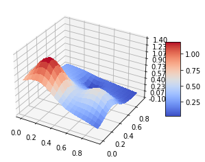
We will first study how to fit polynomials to a specific two-dimensional function called Franke’s function. This is a function which has been widely used when testing various interpolation and fitting algorithms. Furthermore, after having established the model and the method, we will employ resamling techniques such as cross-validation and/or bootstrap in order to perform a proper assessment of our models. We will also study in detail the so-called Bias-Variance trade off.
The Franke function, which is a weighted sum of four exponentials reads as follows
The function will be defined for \(x,y\in [0,1]\). Our first step will be to perform an OLS regression analysis of this function, trying out a polynomial fit with an \(x\) and \(y\) dependence of the form \([x, y, x^2, y^2, xy, \dots]\). We will also include bootstrap first as a resampling technique. After that we will include the cross-validation technique. As in homeworks 1 and 2, we can use a uniform distribution to set up the arrays of values for \(x\) and \(y\), or as in the example below just a set of fixed values for \(x\) and \(y\) with a given step size. We will fit a function (for example a polynomial) of \(x\) and \(y\). Thereafter we will repeat much of the same procedure using the Ridge and Lasso regression methods, introducing thus a dependence on the bias (penalty) \(\lambda\).
Finally we are going to use (real) digital terrain data and try to reproduce these data using the same methods. We will also try to go beyond the second-order polynomials metioned above and explore which polynomial fits the data best.
The Python code for the Franke function is included here (it performs also a three-dimensional plot of it)
from mpl_toolkits.mplot3d import Axes3D
import matplotlib.pyplot as plt
from matplotlib import cm
from matplotlib.ticker import LinearLocator, FormatStrFormatter
import numpy as np
from random import random, seed

fig = plt.figure()
ax = fig.gca(projection='3d')

# Make data.
x = np.arange(0, 1, 0.05)
y = np.arange(0, 1, 0.05)
x, y = np.meshgrid(x,y)


def FrankeFunction(x,y):
    term1 = 0.75*np.exp(-(0.25*(9*x-2)**2) - 0.25*((9*y-2)**2))
    term2 = 0.75*np.exp(-((9*x+1)**2)/49.0 - 0.1*(9*y+1))
    term3 = 0.5*np.exp(-(9*x-7)**2/4.0 - 0.25*((9*y-3)**2))
    term4 = -0.2*np.exp(-(9*x-4)**2 - (9*y-7)**2)
    return term1 + term2 + term3 + term4


z = FrankeFunction(x, y)

# Plot the surface.
surf = ax.plot_surface(x, y, z, cmap=cm.coolwarm,
                       linewidth=0, antialiased=False)

# Customize the z axis.
ax.set_zlim(-0.10, 1.40)
ax.zaxis.set_major_locator(LinearLocator(10))
ax.zaxis.set_major_formatter(FormatStrFormatter('%.02f'))

# Add a color bar which maps values to colors.
fig.colorbar(surf, shrink=0.5, aspect=5)

plt.show()
5.6.1. Exercise: Ordinary Least Square (OLS) on the Franke function
We will generate our own dataset for a function \(\mathrm{FrankeFunction}(x,y)\) with \(x,y \in [0,1]\). The function \(f(x,y)\) is the Franke function. You should explore also the addition of an added stochastic noise to this function using the normal distribution \(N(0,1)\).
Write your own code (using either a matrix inversion or a singular value decomposition from e.g., numpy ) or use your code from homeworks 1 and 2 and perform a standard least square regression analysis using polynomials in \(x\) and \(y\) up to fifth order. Find the confidence intervals of the parameters (estimators) \(\beta\) by computing their variances, evaluate the Mean Squared error (MSE)
and the \(R^2\) score function. If \(\tilde{\hat{y}}_i\) is the predicted value of the \(i-th\) sample and \(y_i\) is the corresponding true value, then the score \(R^2\) is defined as
where we have defined the mean value of \(\hat{y}\) as
Your code has to include a scaling of the data (for example by subtracting the mean value), and a split of the data in training and test data. For this exercise you can either write your own code or use for example the function for splitting training data provided by the library Scikit-Learn (make sure you have installed it). This function is called \(train\_test\_split\). You should present a critical discussion of why and how you have scaled or not scaled the data.
It is normal in essentially all Machine Learning studies to split the data in a training set and a test set (eventually also an additional validation set). There is no explicit recipe for how much data should be included as training data and say test data. An accepted rule of thumb is to use approximately \(2/3\) to \(4/5\) of the data as training data.
You can easily reuse the solutions to your exercises from week 35 and week 36.
5.6.2. Exercise: Bias-variance trade-off and resampling techniques
Our aim here is to study the bias-variance trade-off by implementing the bootstrap resampling technique.
With a code which does OLS and includes resampling techniques, we will now discuss the bias-variance trade-off in the context of continuous predictions such as regression. However, many of the intuitions and ideas discussed here also carry over to classification tasks and basically all Machine Learning algorithms.
Before you perform an analysis of the bias-variance trade-off on your test data, make first a figure similar to Fig. 2.11 of Hastie, Tibshirani, and Friedman. Figure 2.11 of this reference displays only the test and training MSEs. The test MSE can be used to indicate possible regions of low/high bias and variance. You will most likely not get an equally smooth curve!
With this result we move on to the bias-variance trade-off analysis.
Consider a dataset \(\mathcal{L}\) consisting of the data \(\mathbf{X}_\mathcal{L}=\{(y_j, \boldsymbol{x}_j), j=0\ldots n-1\}\).
Let us assume that the true data is generated from a noisy model
Here \(\epsilon\) is normally distributed with mean zero and standard deviation \(\sigma^2\).
In our derivation of the ordinary least squares method we defined then an approximation to the function \(f\) in terms of the parameters \(\boldsymbol{\beta}\) and the design matrix \(\boldsymbol{X}\) which embody our model, that is \(\boldsymbol{\tilde{y}}=\boldsymbol{X}\boldsymbol{\beta}\).
The parameters \(\boldsymbol{\beta}\) are in turn found by optimizing the means squared error via the so-called cost function
Here the expected value \(\mathbb{E}\) is the sample value.
Show that you can rewrite this as
Explain what the terms mean, which one is the bias and which one is the variance and discuss their interpretations.
Perform then a bias-variance analysis of the Franke function by studying the MSE value as function of the complexity of your model.
Discuss the bias and variance trade-off as function of your model complexity (the degree of the polynomial) and the number of data points, and possibly also your training and test data using the bootstrap resampling method.
Note also that when you calculate the bias, in all applications you don’t know the function values \(f_i\). You would hence replace them with the actual data points \(y_i\).
5.6.3. Exercise: Cross-validation as resampling techniques, adding more complexity
The aim here is to write your own code for another widely popular resampling technique, the so-called cross-validation method. Again, before you start with cross-validation approach, you should scale your data.
Implement the \(k\)-fold cross-validation algorithm (write your own code) and evaluate again the MSE function resulting from the test folds. You can compare your own code with that from Scikit-Learn if needed.
Compare the MSE you get from your cross-validation code with the one you got from your bootstrap code. Comment your results. Try \(5-10\) folds. You can also compare your own cross-validation code with the one provided by Scikit-Learn.
5.6.4. Exercise: Ridge Regression on the Franke function with resampling
Write your own code for the Ridge method, either using matrix inversion or the singular value decomposition as done in the previous exercise. Perform the same bootstrap analysis as in the Exercise 2 (for the same polynomials) and the cross-validation in exercise 3 but now for different values of \(\lambda\). Compare and analyze your results with those obtained in exercises 1-3. Study the dependence on \(\lambda\).
Study also the bias-variance trade-off as function of various values of the parameter \(\lambda\). For the bias-variance trade-off, use the bootstrap resampling method. Comment your results.
5.6.5. Exercise: Lasso Regression on the Franke function with resampling
This exercise is essentially a repeat of the previous two ones, but now with Lasso regression. Write either your own code (difficult and optional) or, in this case, you can also use the functionalities of Scikit-Learn (recommended). Give a critical discussion of the three methods and a judgement of which model fits the data best. Perform here as well an analysis of the bias-variance trade-off using the bootstrap resampling technique and an analysis of the mean squared error using cross-validation.
5.6.6. Exercise: Analysis of real data
With our codes functioning and having been tested properly on a simpler function we are now ready to look at real data. We will essentially repeat in this exercise what was done in exercises 1-5. However, we need first to download the data and prepare properly the inputs to our codes. We are going to download digital terrain data from the website https://earthexplorer.usgs.gov/,
Or, if you prefer, we have placed selected datafiles at https://github.com/CompPhysics/MachineLearning/tree/master/doc/Projects/2021/Project1/DataFiles
In order to obtain data for a specific region, you need to register as a user (free) at this website and then decide upon which area you want to fetch the digital terrain data from. In order to be able to read the data properly, you need to specify that the format should be SRTM Arc-Second Global and download the data as a GeoTIF file. The files are then stored in tif format which can be imported into a Python program using
scipy.misc.imread
---------------------------------------------------------------------------
NameError                                 Traceback (most recent call last)
<ipython-input-10-d985fb40c43d> in <module>
----> 1 scipy.misc.imread

NameError: name 'scipy' is not defined
Here is a simple part of a Python code which reads and plots the data from such files
import numpy as np
from imageio import imread
import matplotlib.pyplot as plt
from mpl_toolkits.mplot3d import Axes3D
from matplotlib import cm

# Load the terrain
terrain1 = imread('SRTM_data_Norway_1.tif')
# Show the terrain
plt.figure()
plt.title('Terrain over Norway 1')
plt.imshow(terrain1, cmap='gray')
plt.xlabel('X')
plt.ylabel('Y')
plt.show()
If you should have problems in downloading the digital terrain data, we provide two examples under the data folder of project 1. One is from a region close to Stavanger in Norway and the other Møsvatn Austfjell, again in Norway. Feel free to produce your own terrain data.
Alternatively, if you would like to use another data set, feel free to do so. This could be data close to your reseach area or simply a data set you found interesting. See for example kaggle.com for examples.
Our final part deals with the parameterization of your digital terrain data (or your own data). We will apply all three methods for linear regression, the same type (or higher order) of polynomial approximation and cross-validation as resampling technique to evaluate which model fits the data best.
At the end, you should present a critical evaluation of your results and discuss the applicability of these regression methods to the type of data presented here (either the terrain data we propose or other data sets).